
	Advertisement

Linear Regression

What’s the best way to draw a line through a collection of points?

Let me be a little more specific. Let’s say you are running an experiment in which there are a series of inputs, each of which generates an output which you measure. You want to determine the correlation between the inputs and the outputs.

Mathematicians like to describe values as either dependent variables or independent variables. Independent variables are the inputs (or causes) of the experiment, and the outputs are described as dependent variables (they are “dependent” on the outcome of the experiment).

In our example we’ve decided we are looking for a direct (proportional) relationship. We want to draw a line through the points. We’re looking for a linear correlation.

The fancy, statistical, word for estimating the relationships between independent and dependent variables is called Regression.

Since we are looking for a straight line to draw between the points we want to perform Linear Regression

Data

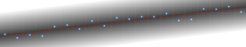
There are an infinite number of lines that can be drawn through a collection of points. Some are obviously better than others. What we want is a way to judge (measure) the quality of each line, then attempt to maximize the quality of the line.

If we can write an equation for a test line, and how this scores using the data points, we can use our old friend, Calculus, to find the optimal solution for the line.

Let’s imagine we have a series of n points.

Each of these is depicted by a pair of coordinates (x_i,y_i)

So, let's find the equation for our line …

Back to School

OK, first we need to visit our old geometry classroom. We need to remember how to describe lines.

A line on a 2D plane can be described using just two parameters. There are numerous ways of doing this, but considering that we’re going to be using Cartesian (x,y) coordinates to describe the data points, let’s select an equation form that simplifies our math.

A line can be described by the gradient which I’ll call M …

… and by the intercept which I’ll depict with C.

The gradient is the ratio of the change in y-values over the change in x-values, and the intercept is the value at with the line crosses the y-axis (x=0).

I’m sure this is all coming flooding back to you.

Errors and residuals

The best-fit line we’ll be searching for can be described using just these two parameters.

What we need to do is find the best M and C for the job, so we need to have some measure of quality to optimize.

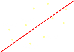
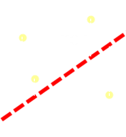
Unless all our test points are already in a perfect line (trivial solution), there will be an error between the value predicted by the line, and the observed dependent variable. These differences are called residuals.

What we want is to find a line for which the total of the residuals between all the points and the proposed line is at a minimum. Using just the sum of all the residuals has two problems: The first is that some of the residuals are positive (above the line), and some are negative (below the line). If we simply added the residuals together, these may cancel out! The second issue is that there is no penalty for a large residual. We want to make sure that points further away from the line suffer more severe consequences.

The solution to both these problems is to square the residuals.

(real) Square numbers are always positive (solving the first issue), plus the penalty of squaring provides the punishment needed for outliers. (A point that is twice as far away from the line has four times the residual penalty, one that is three times as far away has nine times the penalty …)

If we sum up the squares of the residuals of all the points from the line we get a measure of the fitness of the line. Our aim should be to minimize this value.

This is called an (Ordinary) Least Squares Fit.

One more step, and we'll be ready for our Calculus!

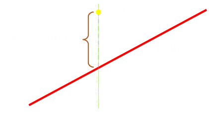
Our independent variable is x, and for every observed dependent variable result y_i there is a corresponding point on the line.

We can calculate the residual error by subtracting the predicted value of y (calculated from the line equation) from the measured value y_i, since we know they both occur at x_i.

The Math

OK, if you're a little math squeamish, you might want to skip past this section.

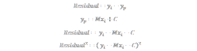
As mentioned above, we can calculate the residual as the vertical descender from the point to the line.

We can substitute the equation of the line and the square the result. This is the square of the residual

To calculate the sum of square residuals, we add all the individual square residuals together. We'll give this sum the symbol Q

All we have to do is minimize this equation and we have our solution! Recalling back to Calculus, the minimum value for Q has to occur when its first derivative is zero. To be at a minimum (or maximum), the gradient of the curve at that point needs to be flat.

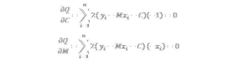
Below are the partial derivatives for Q with respect to the two parameters of the regression line M and C. (I used the chain rule). We want these to be zero to get our minimum.

These two equations can be expanded out to give these two results (respectively):

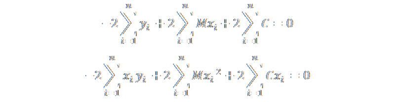
A little more shuffling and dividing by two gives couple of more pleasing-to-the-eye equations:

Finally, we can pull some constants out infront of the sumations. This has some really interesting consequences. The second item in the top equation, simplifies to just nC. We can also pull out M from infront of the sum of the x-values. All the other values we need in order to calculate the regression are similarly simple to calculate.

Finally, some simple substitutions between the two equations (we have two equations and two unknowns) reveals what we want:

There we have it! The equations to calculate the least squares linear regression line through n points.

The equations themselves are very elegant. If you look closely, to calculate a regression line we don't need to remember and store all the coordinate pairs, instead we just need to keep track of a couple derived totals. We can even keep these as running totals that are updated as new points are added or deleted.

In addition to keeping track of the total number of points, all we need to track are: Sum of all x-values, Sum of all y-values, Sum of all xy-products, Sum of all x-values squared, and Sum of all squares of x-values (notice the important, and subtle, difference in the last two?)

More Geek

Another fascinating point about these equations is that the lower equation is based, essentially, on the average (arithmetic mean) value of the recorded y-coordinates and x-coordinates.

Yes, that's right! The least squares linear regression line always passes through the mean of both variables!

Try it for yourself

Below is an interative application based on the principles described above. Use the mouse to click and add points to the graph (or tap if you are using a tablet). Once two or more points are added, the best-fit least squares regression line will be displayed.

If you have the luxury of a right-mouse button you can move the cursor close to a point, it will turn red, and you can right-click to selectively delete that point. There is also a button on the lower left to delete all the points. There is a limit of 100 active points.

Finally, the second button allows you to toggle the descenders. These bars show the residual errors. It is the sum of the squares of these values that is being minimized.

Alternate representation of residuals

An alternate visualisation of the least squares errors is shown below. In this interaction a couple of random points have been chosen for you and the regression line drawn (in gray). Using the mouse you can change, within limits, the parameters of another line to see it's effect on the least squares. This alterntive line is rendered in red.

The Least squares value is shown here as a selection of squares based with sides equal to each residual. The best fit line occurs when the combined area of all the drawn squares is at a minimum. You can see how changing the gradient or intercept of the line might reduce the area of some of the squares, but increases the areas of others. It is only when the red line is drawn over the gray regression line that the area is the minimum.

When the mouse is in the middle of the screen, the two lines should correspond. Moving the pointer up and down the screen, increases and decreases the intercept of the red line. Moving the pointer left and right adjusts the gradient of the red line.

The random button redraws the picture with different data points to experiment with, and the [+] and [–] buttons can be used to increase and decrease the number of points rendered.

Uses of Linear Regression

There are so many applications of least-squared linear regression that to mention just one would do an injustice to all the other applications. You’ve probably used it many times yourself in Excel to fit straight trend lines in data.

Watch out

Whilst Linear regression is very cool, its not always the correct tool for the job. Before using it, you need to understand its limits. There are some problems. The first is that, whilst minimizing residuals is good for the data pattern of trying to fit a straight line, if your underlying data relationship is not a proportional relationship, sure you'll get a line, but this line might not be a meaningful result.

Below are a famous series of four graphs, constructed by the Cambridge statistician Francis Anscombe. They are now known as "Anscombe's Quartet". They serve a reminder that it is often very important to graph data before analyzing it! Outliers and patterns can have a great influence on the data.

In each of the graphs below, the line of linear regression is the same (to 2-3 decimal places).

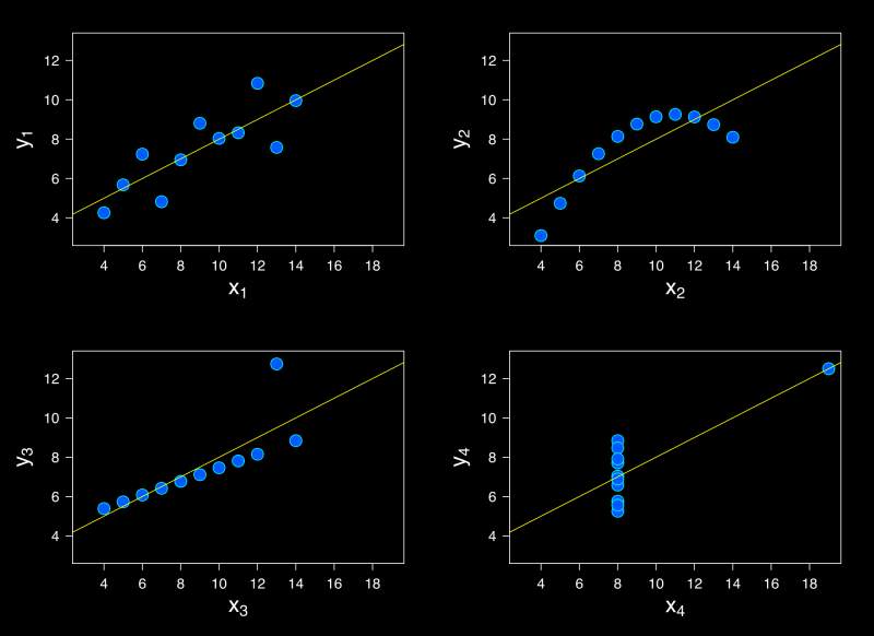
Not only are the regression lines the same, but so are many other properties of the data!

Property	Value
Mean of x in each case	9 (exact)
Variance of x in each case	11 (exact)
Mean of y in each case	7.50 (to 2 decimal places)
Variance of y in each case	4.122 or 4.127 (to 3 decimal places)
Correlation between x and y in each case	0.816 (to 3 decimal places)
Linear regression line in each case	y = 3.00 + 0.500x (to 2 and 3 decimal places, respectively)

Two dependent variables?

Our assumption in deriving the least squares formula was that one of the variables was dependent, and the other independent. This is why we measured the residuals as vertical descenders, and minimized these values. However, this isn't the only approach. We could, for instance, have selected to optimize the horizontal differences, or even the perpendicular distance.

Below are two snap shots from the interactive tool above. In one, I've place two points on the left, and three on the right. In the other, I've place two on the top, and three on the bottom. This 90° rotation is essentially the same thing as switching the algorithm from horizontal to vertical residuals. Can you see the issue?

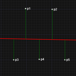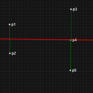If we regard each data point (x,y) as a sample, and if we assume the sample is taken at the precise value of the independent variable x, then it is sensible to regard each data point as being at the exactly correct x coordinate, and all the error is in the sampled value of the dependent coordinate y. On the other hand, if there is some uncertainty in the value of x for each sample, then conceptually it could make sense to take this into account when performing the regression to get the "best" fit.

If both values are equally dependent, it is tempting to suggest using the perpendicular distance as the value to be squared and minimized. This technique is called Total Least Squares, and is also very cool. You can read more about it here. The equations are a little more complex to derive, but not much more.

If both variables are of the same scale and range, this technique can be very valuable, but what if the x and y values are of very different ranges and scales (or distributions of errors)? A delta of one-unit in the x-plane might be substantially more significant to the same unit shift in the y-plane, in which case the perpendicular measure will unfavorably bias one variable.

What if the x and y axes are depicting values of totally different dimensional breakdowns (such as distance on one axis, and time on another?), how can errors in one be compare to the other?

In order to make the best fit, we need to scale the plot axes (conceptually) such that the variances of the errors in the x and y variables are numerically equal. Once we have done this, it makes sense to treat the results as geometrical points and find the line that minimizes the sum of squares of the perpendicular distances between the points and the line. Of course, this requires us to know the variances of the error distributions.

There's more to this straight line stuff than you think …

You can find a complete list of all the articles here. Click here to receive email alerts on new articles.