
Candyland®
 |
This blog concerns the mathematical analysis of Candyland®, a children’s game produced by Hasbro (before that Milton Bradley). The original game was designed by Eleanor Abbot in 1945. Over the years, subtle rule changes have been made. This analysis is based on the rules in the version of the game that our family owns! |
Before reading this article, if you have not done so already, you might want to read the previous two articles regarding the analysis of Chutes and Ladders and Risk. These will set some context.
The Game
There is no skill required to play Candyland (other than being able to recognise colours). A deck of movement cards it shuffled, and players take turns to move their tokens according to the instructions on the card.
The board consists of a linear track containing 134 spaces, mostly coloured red, green, blue, yellow, orange or purple. In addition there are six pink spaces containing named characters, two bridges, and three of the coloured spaces are sticky (more of this later).
Players alternate in drawing movement cards, most of which show one of six colours, and then moving their token ahead to the next space of that colour. Some cards have two marks of a colour, in which case the player moves his or her marker ahead to the second-next space of that colour. The deck has one pink card for each named location, and drawing such a card moves a player directly to that board location (This move can be either forward or backward). Finally, if a player lands on one of the sticky spaces, he misses his next turn.
Landing on the start space to one of the two bridges allows the player to take a short cut. The rules are not explicit about where/how the player moves on a bridge, but in our house, landing on the bridge places you in limbo on the bridge at the end of that turn, and the turn of your next card on your subsequent move determines your destination past the exit of the bridge.
The first player to the last space on the board is the winner.
The Board
My first task was to model the board. There are 134 Visible spaces on the board, which can be stored as a simple array. In addition, there is a space at index zero for the starting location (players start off the board). I modeled the bridges as their own state (when a player is on a bridge, they are on either space 135 or space 136). Finally, to represent the sticky locations, there are three additional ‘hidden’ squares 137-139, one behind each sticky location. Landing on a sticky location, moves the player to this square for their ‘missed turn’, then they move forward on their next round.
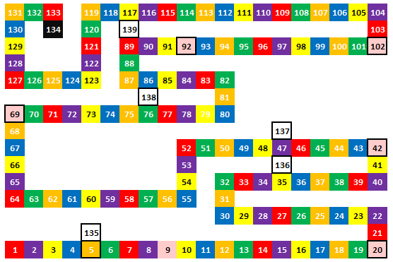 |
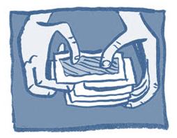
First I created a quick stylised map in Excel (shown on the left) from the game board (shown below). This enabled me to enter the data for the cell colours into an array. 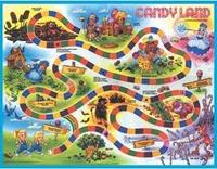
|
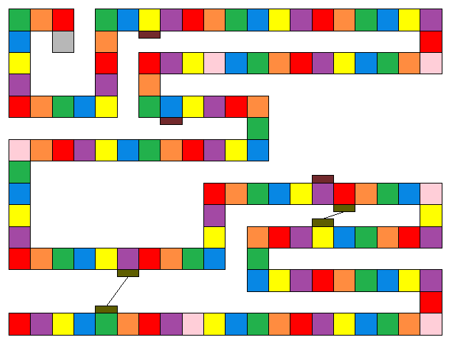
Once done, I could then get code to render the picture:
Distribution of cards
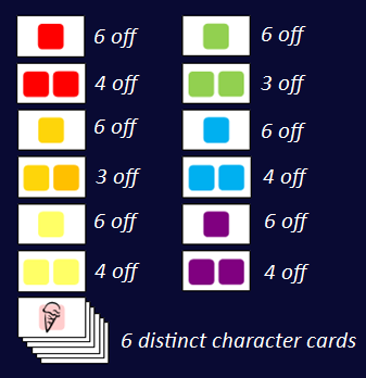 |
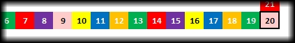
I counted the distribution of cards in the game. Assuming my children had not lost any, there were 64 cards supplied in our version of the game. |
Crippled Markov Chain
The previous systems I have analysed with stochastic Markov chains (RISK dice battles, and Chutes & Ladders) have been Memoryless; The probability of moving to different states has been agnostic as to events that have happened in the past. This is not the case with Candyland.
As cards are drawn, they are used and discarded and so the probability of which card will be turned up next is dependent on cards that have already been seen. (This is easy to confirm with a thought experiment: For instance, if all four double red cards have already been played, the probability that the next unseen card is also a double red will be zero). To work through every possible combination of ways that the cards could be arranged in the deck is computationally infeasible.
Approximation
|
I’m going to make a simplification to turn the system back into a memoryless stochastic system. (We’ll check later on how good this approximation is). How I’m going to simplify the system is that at after a draw and acting on the card, we replace it back into the deck and shuffle. At each draw, there are always 64 cards in the deck, and so a 1/64 chance of drawing any distinct card (essentially making every draw just like the first draw). Yes, it does mean that it is mathematically possible to draw the same card again (especially dangerous when drawing one of the special pink cards, meaning that a player could be sent back more than once), but I’m assuming the probabilities of these events occurring will be ‘noise’ compared to the main probabilities, especially in short games. (In longer games, which sometimes happen, all the cards in the deck are used up anyway and need to be reshuffled, so this results in the same situation). |
 |
Transition Matrix
The transition matrix (for explanation of a transition matrix, review the posting about Chutes and Ladders) for this game is 140x140, with each element (i, j) describing the probability of a player moving from location i to location j on the next move. There is a row/column for each of the visible squares on the board, as well as locations for the ‘hidden’ states (the start, the bridges, and the temporary sticky states ‘behind’ on the three licorice spaces)*
By stochastic definition, the sum of all the probabilities in a row adds up to 1.0 — Something has to happen on each iteration.
 |
*Yes, yes, I know that we can reduce the size of matrix slightly by reducing the redundant rows and columns associated with the start of the bridges. |
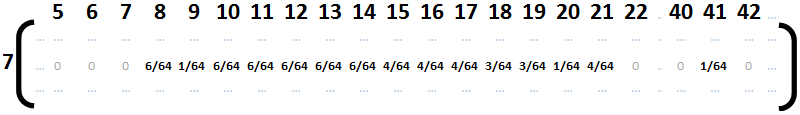
A snippet of the transition matrix is shown below for the follow section of board.
If the player is currently on square 7 there is a 6/64 chance of drawing a Single Purple card and moving to square 8. Square 9 is a special pink character, and there is only a 1/64 chance of drawing the unique character card for this space. (Similarly 20 and 42 and all the other pink squares.)
Squares 10-14 are also reachable with single cards with probability 6/64. Further out, the squares that are accessible with double cards have different probabilities because of their different frequencies in the deck.
With care it is possible to construct a transition matrix for the game which enumerates the probabilities of moving from every game state to every other game state.
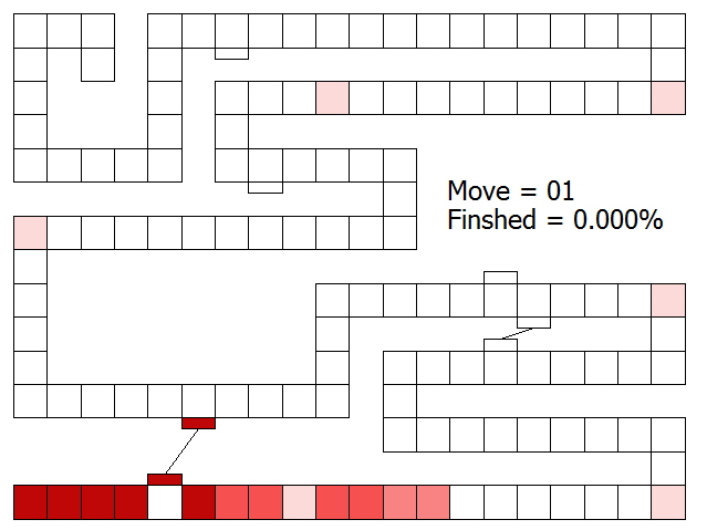
All that is needed now, is to create a column identity vector with 1.0 in row zero and the rest zeros (all games are started with the player token off the board with 100% certainty!), and multiply this by the transition matrix. The row vector output will show the probability distribution for where the player token could be after one card draw. Below are the results represented in graphical form, with shading denoting the probabilities. Darker red representing high probabilities and Lighter red representing low probabilities.
After one draw, the darkest areas are, obviously, the ones that are reached by the cards that have the highest distribution in the deck (the single colours). The spaces obtained by the double colours are lighter shaded (some lighter than others because there are less of these cards in the deck). You can see that it is possible to reach the first bridge with a single green, and each of the special pink locations is shaded very light to represent the 1/64 chance of turning up the special character card for that location. It’s not possible to complete the game in one move, so the percentage chance to finish is 0.000%
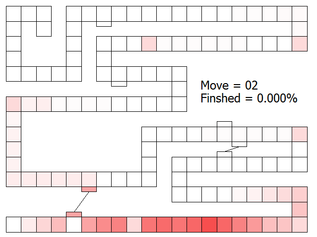
If we multiply the above output vector by the transition matrix again, the new output vector represents the superposition of probabilities of where the player token could be after the second drawn card (starting from all the weighted starting positions of the first vector). The result is shown below. The probability ‘cloud’ is thinning out a little, and the most probable space is the red square 14 (I’ll leave it as an exercise to the reader to convince themselves why this would be the case). The pink squares are the same shade, and there is still no way to reach the finish line with just two card draws. You can see a second probability ‘cloud’ appearing downstream of the first bridge (and also very, very faint clouds downstream of each pink square, but these are so faint that contrast does not allow the eye to differentiate them from white using the shading scheme I’m using here).
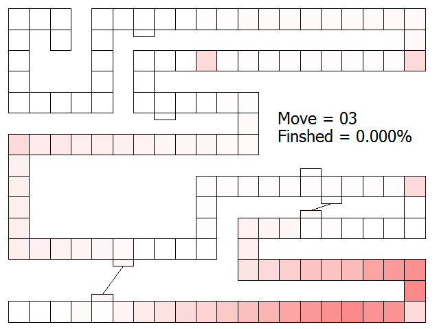
After the third card draw, the probability distribution looks like the picture below. The clouds are getting wider, and more of the board is shaded. (It’s possible now that the second bridge might have been used).
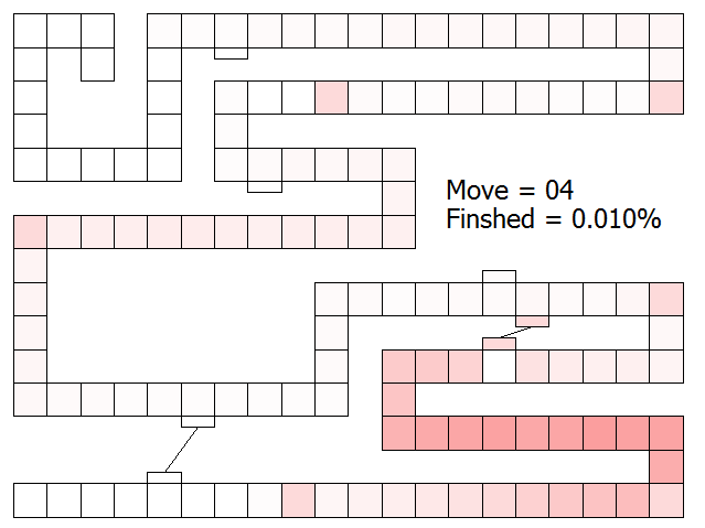
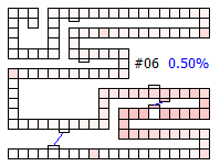
After four draws, and interesting event occurs — it is mathematically possible to win the game! (The probability of landing of finishing the game in just four moves is approximately once in every 10,000 games). There are multiple ways to achieve this victory, but all require that the first card drawn be the pink special card that takes the player to square 102. (In our version of the game, this is the Ice Cream).
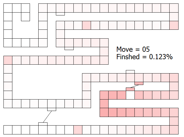
By five draws, there are more ways to achieve the victory condition as you can see from the probability increase of the token being on the finish space.
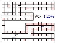
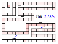
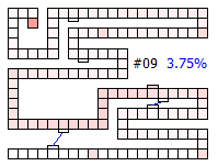
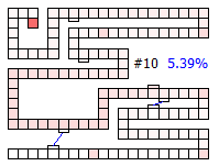
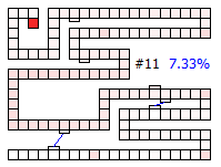
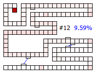
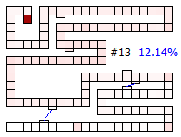
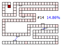
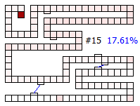
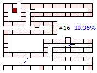
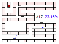
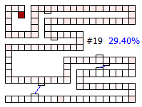
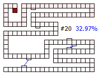
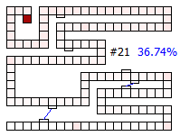
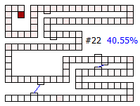
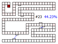
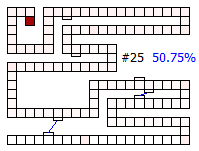
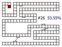
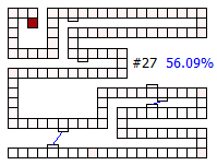
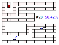
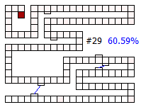
Below are thumbnails of the board showing the percentage of finishing increasing with each drawn card.
 |
 |
 |
 |
 |
 |
 |
 |
 |
 |
 |
 |
 |
 |
 |
 |
 |
 |
 |
 |
 |
 |
 |
 |
Animation
 |
Here is a short video animation showing the probability distribution for the first 50 card draws. |
How long is an ‘average’ game?
Below is a graph of the probability of a single person finishing the game by move-n.
99.2% of games will finish within 100 card draws.
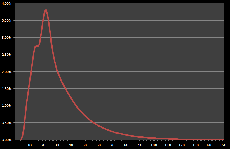
The Modal number of card draws to is 22 . (More games will finish using this number of moves than any other number).
The Median number of card draws to is 25 . (Half the number of games will be shorter than this, and half longer).
The Arithmetic Mean (average) number of card draws to is 30.56 (If you play N games, on average, you’ll draw N*30.56 cards).
How good an approximation is our simplification?
I was curious to learn just how close the replace-and-reshuffle simplification to the model was to real results, so I decided run an objective comparison. I created a Monte-Carlo simulation of the game so that I could automate the game and execute it millions of times. (This did not take long to code, as most of the work in creating the first simulation was the data-structures, and serialization of state and this could all be re-used). Another benefit of writing the simulation is that it is possible to model a game with more than one player. There are two reasons why this is important: |
 |
1) |
When there are more players, more cards are drawn, so it is much more likely that the deck will need to be reshuffled (sometimes many times). Reshuffling creates the situation that the special pink cards are encountered multiple times. |
2) | In real-life, a game ends when the first person crosses the finish line. With multiple players, there are multiple chances for the game to end in a round. |
Quick Compare
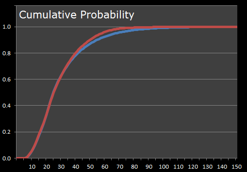
Here I've plotted the results of The Markov Chain Analysis and Monte-Carlo Simulation (100,000,000 games) on the same chart.
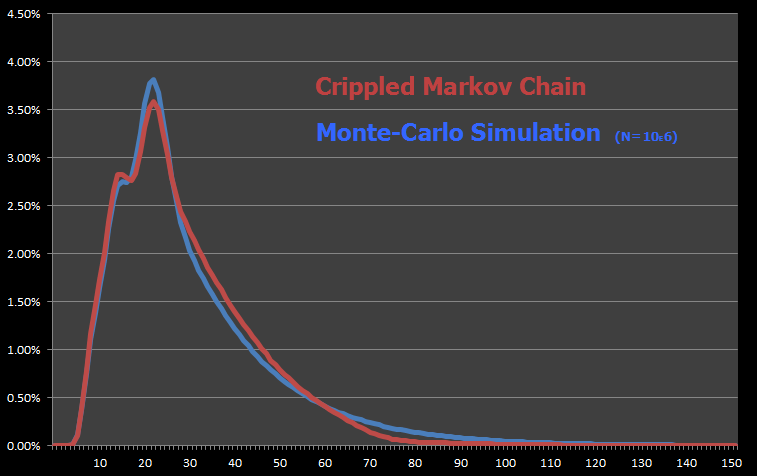
They look pretty close! This is a good thing, and shows that we've probably not made any simple logic errors in the code — Getting the same results using two different mechansims of calculation always makes one feel warm inside. The fact that the curves are pretty close also confirms that our simplification approximation was a valid one to make.
The 'true' curve, the Monte-Carlo one, peaks a little higher at the mode, which is to be expected. Why? Well, to complete the game in a small number of moves requires the use of one of the pink cards and so these will be used up. Until the deck is reshuffled (post 64 drawn cards), there is zero chance of encountering that pink card again. However, in the Markov Chain model, it is possible to encounter the same pink card again, and encountering the same card twice will send you backwards. This does not happen often, but it does enough to slightly lower the perentage chance at the modal peak.
 |
Another way to look at the data is to view the Cumulative Probability of a game finishing by at least n-moves. As you can see, the simplified Markov model seems to slightly over-estimate the probabilities once about half the deck has been drawn. The Mode and Median of the two methods are the same at 22 and 25 respectively, but the Mean decreases from 30.56 for the Markov approximation to 28.98 for the Monte-Carlo simulation. |
Multiple Players
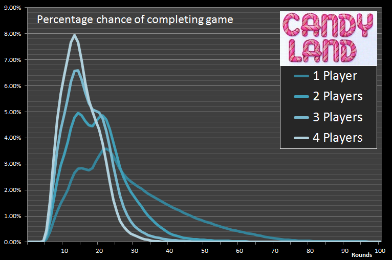
When there is more than one player in a game, the statistics change quite considerably because of the two reasons mentioned earlier.
Below is the graph of the percentage chance of completing a game in n-rounds. Note – Here 'round' refers to each person taking a card, and this is subtly different from drawing cards. With four players in the game, a 'round' uses four times as many cards so the deck reshuffled much more. Remember, the Mean number of cards taken in a single player game is less than half a deck? This means that in half of the single player games, the Ice Cream card (which teleports you most of the way across the board) will never have been select. With four players eating through cards at four times this pace, everytime there is a re-shuffle, it's a certainty that one player used this card.
Here is the same data presented in cummulative probability format.
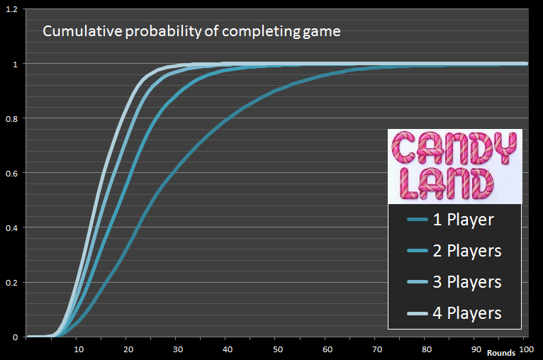
Effect on the averages
Here are the changes to the averages number of rounds, based on the number of players.
| 1 Player | 2 Players | 3 Players | 4 Players | |
|---|---|---|---|---|
| Mode | 22 | 14 | 14 | 13 | Median | 25 | 19 | 16 | 14 | Mean | 28.98 | 19.97 | 16.70 | 14.87 |
You can find a complete list of all the articles here. Click here to receive email alerts on new articles.
© 2009-2013 DataGenetics