
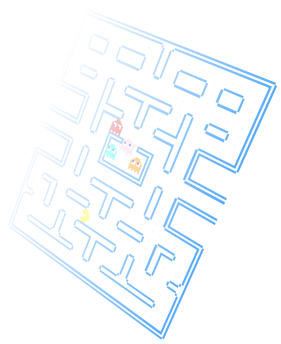
Mazes
In this article I’m going to take a look at one of the many algorithms that can be used to generate mazes. The technique I am going to describe uses a depth first search strategy. It is also given the name of a recursive backtracking algorithm. Both of these names should give you clues as to how the technique works. |
 |
 |
A maze is a complex structure of interconnected passageways. There should be (at least) one way to get from a designated start location to a designated end. Typically the path is convoluted and branched (these branches can also be branched, and often leading to dead-ends) making it not obvious to the naked eye the correct path to take (even when exposed to a God’s eye view from above with all information exposed). Mazes are even more challenging to solve when you are inside one and are only exposed to the information you can immediately see! |
Generating Mazes
Different algorithms for generating mazes work in different ways. Some start with a ‘solid’ block and ‘carve’ out passages as they progress. Others start with an ‘empty’ space and ‘build’ walls. The back track recursive algorithm is a carving algorithm: It starts out as a complete grid with all boundaries and walls set and removes walls to generate the labyrinth. In this article I’m using a 2D rectangular grid but the technique can be generalized to any tessellating shapes in any number of dimensions. |
 |
First, however, let’s take a quick look at ways we can describe mazes:
Properties of mazes
Mazes have characteristics that describe them. A maze is classified as ‘perfect’ if it does not contain loops (as we will see later, the dual of a maze is a graph, and if this graph is a single tree with no cycles then it is a perfect maze. A perfect maze can also be described as a ‘simply connected’ maze.
If a maze is simply connected it is possible to solve it using a wall following algorithm. By always keeping you right hand (or left if you prefer!), against the maze wall and walking around you will walk a path that will eventually visit every location in the maze and return to the same location.
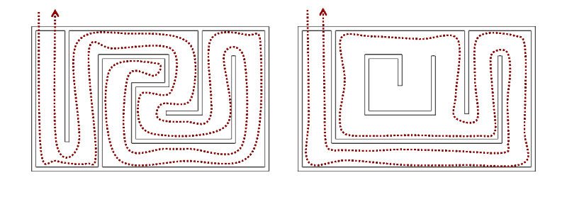
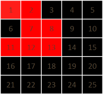
The maze on the left above is a simple maze. By selecting a wall and following it all the way around, each and every location in the maze is visited. Wherever the entrance and exit were, with a simple maze, following a wall will, eventually, take you past them. The maze on the right is not simple; it has a loop (island). Using a wall following algorithm you are not exposed to all locations. If the exit of this maze happend to be in the island, you would never find it using a simple wall follower.
More properties
Mazes are usually generated using random number generators and even running the same algorithm twice in a row (with different seeds for the random number generator) will produce different results. However, on average, different algorithms have different characteristics and properties. Here are some of these characteristics:
Simply connected/Complex - We’ve mentioned this already. Is it possible to visit every location by simply following one wall? If so, the maze is simply connected. A simply connected maze does not have any loops.
Number of dead-ends - It’s possible to make maze that has no wrong turns at all, it’s just a convoluted loop! This would not be a very challenging maze! The number of dead ends in a maze is the measure of the number of locations in the maze that have only one way in. A maze that has only a few dead-ends, and long pathways in-between, might be quite frustrating as you’d have to go a long distance before finding out you’d gone the wrong way!
Length of longest path - This is often measured as percentage. First you find the shortest (optimal) path through the maze, then measure the ratio of the number of cells on this path to all the cells in the maze. A high percentage indicates a fair amount of convolution and twisting of the solution (taking lots of turns in order to get to the destination, and visiting a good measure of the maze before exiting).
Convolution - Either measured as twistiness, or its inverse straightness, and is some metric to measure how often in the maze that the path exits a cell on the opposite side of the way it came in, and how often it turns a corner in a cell. The human brain has an easier job following paths that are straight (if you see a long line a cells in a straight line you instantly know that there is a clear path to the end of this section. However, if the path is twisted, you can’t immediately see to the end and have to trace it to find out).
Distribution of Valency - Dead ends cells have a valency of one (There is only one way in and out of that cell). Crossroads have a valency of four (in a rectangular grid maze); there are four possible directions to go from this cell. Unbranched corridors have a valency of two, and T-junctions have a valency of three. Different maze algorithms generate different distributions of valencies. An algorithm with a high percentage of T-junctions and crossroads exposes the solver to lots of options. One with a high percentage of corridors (valence two cells), takes the user on long ‘rides’.
Complexity - Related to all the above, this is a measure of the average number of ‘decisions’ a solver will have make to get from the start to the end. What is the average number of junctions you’ll encounter when solving a maze?
Mazes can also be described as having biases; these are patterns baked into the maze by the algorithm (typically by modifications to the random number generator). For instance, instead of selecting entirely at random, an algorithm could be programmed to give a much higher probability of turning clockwise when exiting any cell (making obvious twists), or alternatively, configured to have a much higher probability of exiting a cell opposite the way that it came in (making a maze that has a bias for long runs of straight corridors).
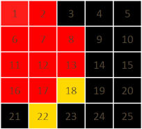
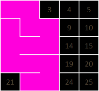
Both of the above mazes are perfect mazes. The one on the right has a strong vertical bias. It also has a high concentration of two valence cells, and high straightness.
Graph Theory
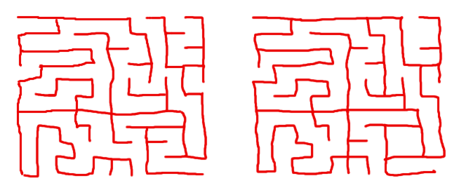
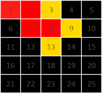
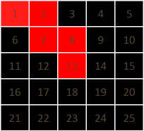
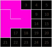
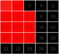
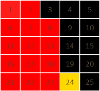
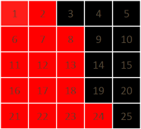
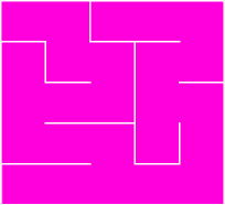
Below are two mazes. The one of the left is a perfect maze, the one on the right has loops. There is an alternate way of thinking about a maze. Instead of thinking about the walls, we can think about the paths between cells. Mathematicians call this a dual network.
The pathways form a graph (sometimes called a tree). The graph for each maze is shown below in red. We can see now that if there is more than one graph the maze is not solvable (if the start and exit are in different trees); this is because there would be no path between the seperate trees.
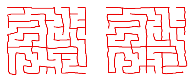
Where the maze has (redundant) loops - representing alternative ways to get to the same location we can see the graph also has loops.
Spanning Tree
 |
From this we can see that to generate a perfect maze what we need to do is create a random spanning tree that connects all the cells in the maze. The various ways of generating spanning trees form the basics of various maze generating algorithms. The one we're going to look at is a recursive backtracking algorithm. |
Recursive Backtracker
 |
The basics of a recursive bactracking algorithm is that we start somewhere on the maze (it does not matter where), and step in a random direction onto a new square. The constraint is that we can't step onto a square that we've already trodden on. When travelling to this new square we remove the wall to the new square and this is what carves out the maze. We keep a track of which squares we've visited and which we have not. We keep repeating this algorithm: Examining all the neigbours of the current square and selecting (at random) any of the unvisited squares, moving into it, then mark this new location as also visited. This is all well and good but sooner or later we'll find that we've painted ourself into a dead end and there will be no neigbouring unvisted squares. What the algorithm does then, is take a step backwards to see if there are any unvisted neigbours from the last visited square, if so carrying on from there, if not, it takes another step further back and looks from there, etc … This keeps going on (moving forward into unvisted squares), or backing up until a square with unvisted neighbours is found, until all squares have been visited. It is called a depth first search because the algorithm plows as far forward as it can before backing up. |
|
A common way to implement this is through the use of a stack (First In Last Out). As we visit each square for the first time, we push this location onto a stack which keeps track of the order we've visited them (a stack is like a stack of plates; it's a list but with strict rules about how we can access them), we keep adding plates to the top (pushing the current location onto the stack) for every forward move we make until we can't make any more moves. When we get stuck, we pop off the top item from the stack (the last visited square), and carry on from there. If the previous location popped off the stack is also blocked, we pop off the next item from the stack (the previous, previous visited location), and so on … The stack dynamically changes in length as the algorithm progresses. |
 |
Let's see this in action …
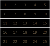 |
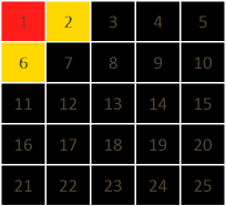
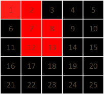
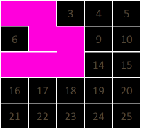
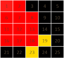
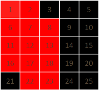
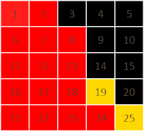
We'll demonstrate this with a small (5x5) maze. The cells are numbered as seen on the left. RED squares are cells that have been visited. The stack is currently empty. All the walls are are currently present between all locations in the grid. |
|
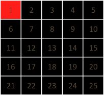 |
Next we select a location to start. This can be random, but let's chose #1. This location is pushed onto the stack. We've visited our first location. STACK: 1 |
|
 |
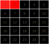
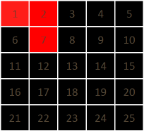
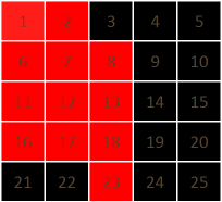
We're currently at grid location #1. Next we enumerate all possible destinations from here. We find out all possible (non-visited) locations that are adjacent to the current location. We'll show these in YELLOW The possible locations are #2 and #6. We'll select one of these at random. |
|
 |
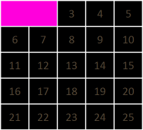
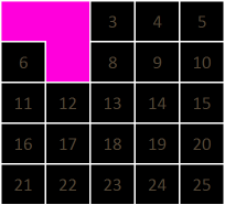
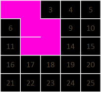
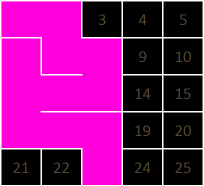
We've selected #2. This location is now pushed onto the stack. We now carve a path between #1 and #2. We do this by removing the wall seperating these two locations. The image on the right shows the maze as it is developing. The Magenta locations have been visited. STACK: 1 2 |
 |
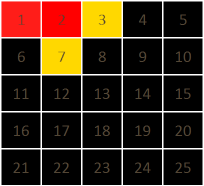 |
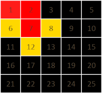
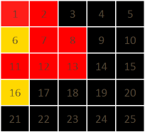
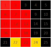
We again enumerate the possible next locations. Again, there are two to select from: #3 and #7. STACK: 1 2 |
|
 |
We've selected #7. This location is now pushed onto the stack. We now carve a path between #2 and #7. STACK: 1 2 7 |
 |
 |
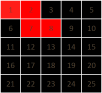
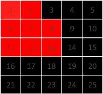
This time there are three possible next locations: #6, #8 and #12. STACK: 1 2 7 |
|
 |
We've selected #8. This location is now pushed onto the stack. We now carve a path between #7 and #8. STACK: 1 2 7 8 The maze is starting to develop! |
 |
 |
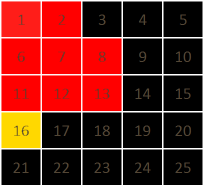
Again there are three possible next locations: #3, #9 and #13. STACK: 1 2 7 8 |
|
 |
We've selected #13. This location is now pushed onto the stack. We carve a path between #8 and #13. STACK: 1 2 7 8 13 |
 |
 |
Again there are three possible next locations: #12, #14 and #18. STACK: 1 2 7 8 13 |
|
 |
We've selected #12. This location is now pushed onto the stack. We carve a path between #13 and #12. STACK: 1 2 7 8 13 12 |
 |
 |
There are two possible next locations: #11 and #17. STACK: 1 2 7 8 13 12 |
|
 |
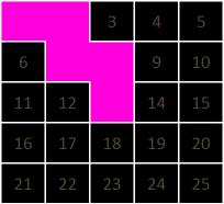
We've selected #11. This location is now pushed onto the stack. We carve a path between #12 and #11. STACK: 1 2 7 8 13 12 11 |
 |
 |
There are two possible next locations: #6 and #16. STACK: 1 2 7 8 13 12 11 |
|
 |
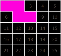
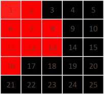
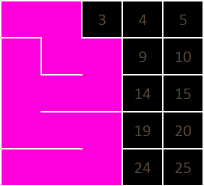
We've selected #6. This location is now pushed onto the stack. We carve a path between #11 and #6. STACK: 1 2 7 8 13 12 11 6 |
 |
|
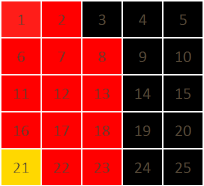
OK, here we have a problem. We're at a dead end. There are no unvisted locations to go from #6. This is where we back track, we pop off the last visited location off the stack. Where were we before last before we go to this location? That's right, we were at #11. STACK: 1 2 7 8 13 12 11 |
|
 |
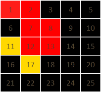
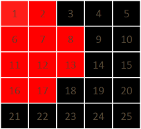
We return to #11. Are there any, yet, unvisted neighbours for #11? Well yes, there is one, and this is #16, so we'll go there. This new location is added to the stack. STACK: 1 2 7 8 13 12 11 16 |
|
 |
And we continue to carve the maze. STACK: 1 2 7 8 13 12 11 16 |
 |
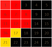 |
There are two possible locations from here: #17 and #21. STACK: 1 2 7 8 13 12 11 16 |
|
 |
#17 is chosen. STACK: 1 2 7 8 13 12 11 16 17 |
 |
 |
There are two possible locations from here: #18 and #22. STACK: 1 2 7 8 13 12 11 16 17 |
|
 |
#18 is chosen. STACK: 1 2 7 8 13 12 11 16 17 18 |
 |
 |
There are two possible locations from here: #19 and #23. STACK: 1 2 7 8 13 12 11 16 17 18 |
|
 |
#23 is chosen. STACK: 1 2 7 8 13 12 11 16 17 18 23 |
 |
 |
There are two possible locations from here: #22 and #24. STACK: 1 2 7 8 13 12 11 16 17 18 23 |
|
 |
#22 is chosen. STACK: 1 2 7 8 13 12 11 16 17 18 23 22 |
 |
 |
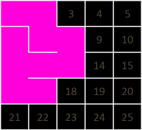
There is only one possible location to go: #21. STACK: 1 2 7 8 13 12 11 16 17 18 23 22 |
|
 |
#21 is added. STACK: 1 2 7 8 13 12 11 16 17 18 23 22 21 |
 |
 |
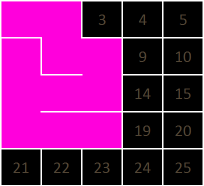
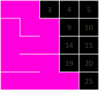
Again we've nowhere to go, so we pop off #21 from the stack. This does not help us either, so we pop off the next value, #22. We're back to #23. There is only one possible location to go from here, and this is #24, so that's where we are heading next. STACK: 1 2 7 8 13 12 11 16 17 18 23 |
|
 |
#24 is added. STACK: 1 2 7 8 13 12 11 16 17 18 23 24 |
 |
 |
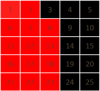
We carry on this process. If you look closely, the stack, as it grows describes the solution to the maze. In fact, whilst we're using backtrack recursion to generate this maze, this same technique can actually be used to solve mazes. STACK: 1 2 7 8 13 12 11 16 17 18 23 24 |
|
 |
The stack will continue to increase and decrease in size as cells are added to the completed maze. Eventually, all the locations in the maze will be visited, and cells will be continuously popped off the stack as we confirm this. When the stack has reached zero length, we will be back where we started and every cell will have been visited. A stack length of zero is the termination criterion for this algorithm. All finished!
STACK: (empty) |
|
Interactive Demo
The applet below uses the recursive backtracking algorithm to generate perfect mazes. Unvisited squares are coloured orange. Initially all internal walls are present. The START/STOP button can be used to start and pause the algorithm. The current location of the algorithm in the maze is shown with a yellow square. As the algorthim progresses, walls are removed and visited squares turn dark.
The program stops when the maze is complete, or can be manually RESET using the appropriate buttom. If you want to watch the algorithm in more detail, there is a SLOW speed option to the rendering. Finally, underneath the maze is a bar depicting the current size of the stack (This can be optionally displayed using the last button).
As the algorithm moves through the grid (depth first), you will see the stack grow. It will increase in size everytime an unvisited square is encountered, and decrease is it backtracks through already visited locations. The code will terminate when the stack returns to zero (all squares visited).
Want to learn more?

|
If you want to learn more about code to generate (and solve) mazes, as well as details of many of the other algorithms available to generate mazes (of differing geometries and complexities), then I highly recommend a book I read recently: Mazes for Programmers - Code Your own Twisty Little Passages, by Jamis Buck. |
You can find a complete list of all the articles here. Click here to receive email alerts on new articles.

© 2009-2015 DataGenetics Privacy Policy