
Shuffling
|
If you are anything like me, you first learned computer programming for fun. Your first program might have been a "Hello World" program. |
 |
 |
Next you may have written a "I’m thinking of a number, try to guess it" game.(Giving Too High, Too Low feedback responses to the input). After that you might have graduated to writing a game based on a deck of cards. |
|
This would mean that you’d have needed to write a function to randomize a deck of cards. There are various ways of doing this. How did you do it the first time? A lame way is to start with a blank array into which you will insert cards into random positions(Pseudo code below. A value of zero is unfilled, and the cards are numbered 1-52): |
 |
For i = 1 To 52 Do t = Int(Rnd() * 52) + 1 Loop Until Card(t) = 0 Card(t) = i Next i
What this code does is generate a random number for the position to insert the next card, then tries to insert the card into that position. If there is a collision, it backs off and tries to insert that card in another random position, and continues this process until it finds a vacant location. Upon success, it works on the next card, then the next, until all cards have been inserted.
At first, cards go in easily, then, as more cards get inserted, collisions occur more and more often. Eventually it gets really hard. As mentioned before, this algorithm is a little sad (There's not even a guarantee that it will ever finish!) There are many things wrong with this algorithm. There are optimization and modifications and improvements, but it’s just not worth trying to implement. We need to do better.
Shuffling
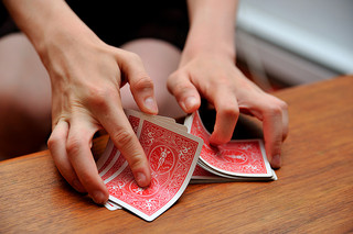 Image: kayray Image: kayray |
Instead of trying to insert cards into random positions into an empty deck container, how about starting with an already full deck (ordered) and shuffle this? This emulates what happens in the real world; we take a deck of cards and swap them around. We can do this in place.
|

Maybe you wrote something like the code below? First it creates a full ordered deck, then it moves through the array once, and swaps the card in that position with another card from a random position:
'Generate deck For i = 1 To 52 Card(i) = i Next i 'Shuffle For i = 1 To 52 s = Int(Rnd() * 52) + 1 'Swap card in position s with that in position i t = Card(s) Card(s) = Card(i) Card(i) = t Next i
I’m ashamed to say, I once wrote code just like this.
This code is terribly, terribly wrong!
It’s one of those things that, at first, you might not see (I had to have it called out to me when I was younger), but once you do see it, you can’t unsee it. As a good programmer, when you see the light, it’s your duty to educate others about this.
So what’s wrong with the code above? It looks so simple; It’s taking a pair of indices and swapping their locations. It’s doing it at random*. There appears to be no logical errors, why is this so terribly bad?
The issue is that this algorithm produces biased results.
*I’m operating under the assumption that we are using a Random Number Generator (RNG) with sufficient precision for the deck of cards we are trying to shuffle (this might not be the case, for reasons that I’ll describe later on).
Even though it appears as though things are being swapped totally randomly, this is not the case. Certain outcomes are much more likely to occur than others because some numbers are being swapped with inappropriate probabilities. Some numbers are getting more chance of being switched than others.
To show what I mean, we’ll start with a more manageable data set, then we’ll expand from there. Let’s consider what happens if we have just three cards:
Three Card Monte
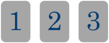 |
Here we have three cards. We load them into an array in order. We now apply the shuffling algorithm from above. We move a pointer over each card in turn, generate a random number from 1-3, and swap the card from that position with the card under the pointer. |
|
On the first pass of the loop (i=1) we randomly switch the card in the first position with any of the other positions. There is a one in three chance the card stays where it is, and each of the other options are equally likely. |
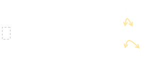 |
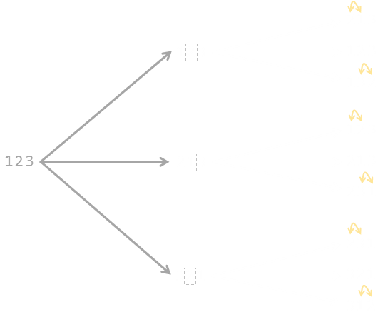
There are three possible outcomes after the first pass of the loop: 123, 213, 321.
One the second pass of the loop (i=2), we randomly switch whatever is in the second position. Here is a tree of the possible outcomes. Again, each of these outcomes is an equally likely to occur.
Finally, we come to the third pass of the loop (i=3). Here is the complete tree:
If you count the number of outcomes, you see that there are 27 equally likely outcomes. Some of these occur more than once. This should already hint at the problem to you …
Since there are just three cards, we know the number of possible permutations is 3! = 6. There are only six ways the cards can be shuffled. These are: 123, 132, 213, 231, 312, 321
|
27 does not divide equally by 6. Oh dear! In fact, to the left is a table of the distributions generated by our bogus algorithm. You can see the the sequences 132, 213 and 231 occur 5/27 (18.5% of the time), whilst all the other numbers occur 4/27 (14.8% of the time). This algorithm generates biased results. We'll look into why a little later, and how to fix it. |
With just three cards, this difference is very noticable. It doesn't get better as the number of cards is increased …
Four apples up on top
If there are four cards, then there are 256 possible ways that our bogus shuffle will arrange the cards, but just 24 permutations they can be arranged (4!)
|
|
This results in a swing from 8/64 (12.5%) to 15/64 (23.4%), with 2143 being almost twice as likely to appear as 4123 or 4231.
Monte Carlo
The good thing about computers is that we can corroborate this theory with simulation. As confirmation, I implemented this bogus algorithm and had it shuffle sets of six cards a million times. We call this a Monte Carlo Simulation.
Here are the results:
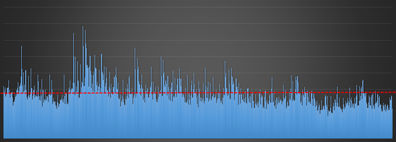
Each outcome is depicted as a bar on the x-axis, in nominally numeric order from 123456 on the left to 654321 on the right. If the shuffling algorithm were a good one we'd expect a fairly uniform distribution of the answers (with a little random noise due to the sample size and the Random Number Generator used) with the blue bars being approximately the same height.
This is not what happens, there is bias in the answers. The more popular answer is occurring nearly five times more often than the least popular answer. The expected value is shown by the red dotted line. This bias is huge. If you were developing a game based on this, it would not be fair (and if a devious person knew about this bias they could exploit it and use this knowledge to their advantage).
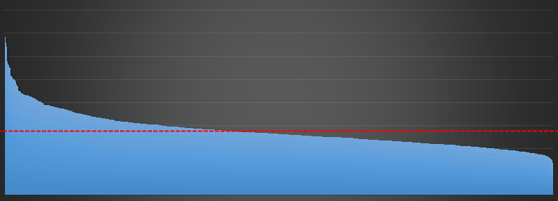
You can see this bias even more clearly if I plot the bars in sorted order:
So What's going on? What causes this bias?
The root cause of this bias is that some items are being given the opportunity to swap more often than others. The loop that passes over the array is swapping items with the the same probability, but as swaps have been made the probability to swap later items needs to change (and the number of items we should consider swapping should reduce). Confused? We can explain all with this little thought exercise.
Imagine we have a deck of cards and we want to shuffle this deck. We'll do this by creating a new deck out of the old deck.
There are initially 52 cards in the source deck. We're going to pick one card at random from this deck, remove it, and this card will be the first card in our new deck. There are 52 cards in the source deck, so we have a 1 in 52 chance of picking any card. After the card is removed, there 51 cards left.
We draw this card, then remove it, and it becomes the first card in our new deck. Two very important things occur here (that the bogus algorithm does not take into account):
Once a card is moved to the new deck, it does not get the opportunity to move back.
The number of cards in the source deck gets fewer with each draw.
When it comes to drawing the second card for our new deck, we have a 1 in 51 chance of taking any of the remaining cards. When we are drawing our third card, then there is a 1 in 50 chance of drawing what is left, and so on …
The probability of drawing cards changes as more cards and drawn, and cards never get chance to be put back in the source pile after being selected. Each card has been appropriately chosen because when it was added into the new deck when there were n cards left to chose from; it was selected with probability 1/n.
Fisher–Yates shuffle
|
The algorithm described above, which is a fair way to shuffle, is called the Fisher–Yates shuffle, named after Ronald Fisher and Frank Yates. (It is also known as the Knuth shuffle after Donald Knuth). |
Rather than keeping arrays for two decks (the source and the destination), an optimisation to this algorithm can be made by swapping cards in-place. This is implemented by keeping a high-water mark representing cards that have already been taken.
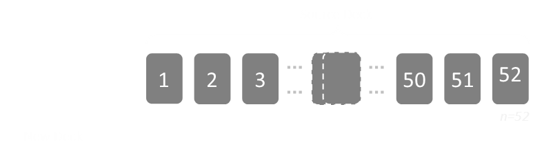
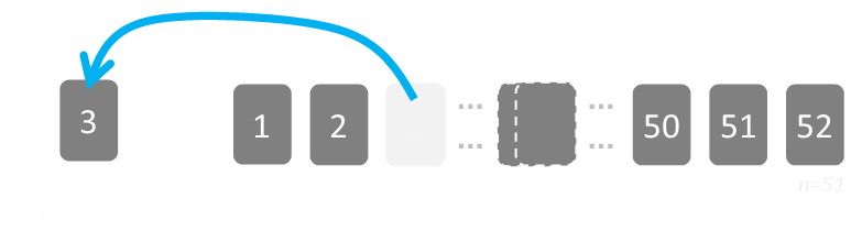
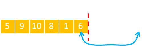
Here is our array, initially sorted. The red line shows the dividing line between what has been fixed and in the new deck, and those not yet selected. Items to the 'left' of the line are in the new deck. Items to the 'right' of the line are still in the source deck.
Initially the deck is all unselected. A card is chosen, and this is shifted into the first ordinal position. A cursor is moved up representing the boundary between those already picked and those remaining. In this way, we don't have a sparse array; we fill the gap with the card that came out with the one displaced from the ordinal position in the new deck.
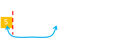
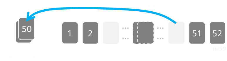
The select card (in this example the 5) was selected by selecting a number from 1-10 as there were 10 unselected cards at the start. It is moved to the front of the array, swapping positions. There are now nine unselected cards, so this time the random number is selected it needs to be from 1-9.
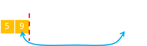
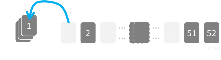
This next selected card is swapped, and the high-water cursor is advanced, reducing the selection from the next card from 1-8.
This process continues until the high water cursor gets to the end (actually, one step away from the end, since when there is only number left, it's certain that it will be swapped with itself!)
Another way to implement this is to move the high water cursor from the right to the left, instead of the left to the right. It's the same thing, but many people prefer to write it this way as the the random number generator just counts between one and the number of yet unselected cards.
Here is some pseudo code for the implementation of this:
'Generate deck For i = 1 To 52 Card(i) = i Next i 'Shuffle For i = 52 To 2 Step -1 s = Int(Rnd() * i) + 1 'Swap t = Card(s) Card(s) = Card(i) Card(i) = t Next i
So, how well does it perform? Using the new algorithm, here is a graph of the results compared to the old bogus code. The blue line is old bad algorithm. The orange line is the graph of the Fisher-Yates shuffle over a million shuffles.
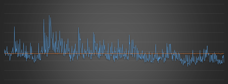
This is much more what we'd expect with from a shuffle! A good distribution with no bias, and just a little noise. If we think back to the very first insert algorithm we suggested at the beginning of this article, maybe we were being unnecessarily cruel when we called it 'lame'. It did, after all, produce a good unbiased shuffle, it's just that it was inefficient in dealing with collisions and sparseness. The Fisher-Yates does a hybrid thing. It is inserting cards without replacement and handling the sparseness by moving the cards into a gap and keeping track of what has been selected and which has not.

Proof
Below is a tree diagram of the Fisher-Yates algorithm in action for a set of three cards.
Initially, the outer loop i=3 means it is the card in the last position we are going to switch. As it is the first pass, the value we can switch with is any of the other positions, so the random number is from 1-3.
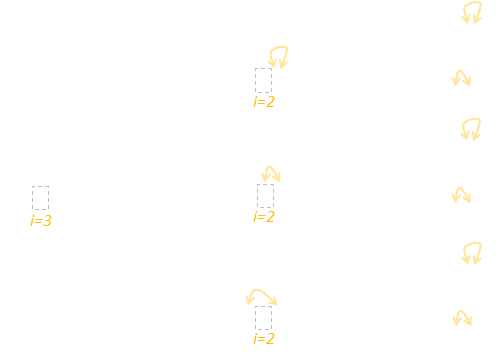
On the second pass, the value in the last position is fixed (never to be changed again). We're determining which card to place in the middle position i=2. There are only two possible options.
There is no reason to run a third pass, as there is only one number remaining un-chosen. You can see there are exactly six answers on the right (each of equal probability), which is the 3! we expect.
Distribution of bias
Another thing we can look at is the distribution of the bias to see if there are any patterns.
If we shuffle a deck of cards lots of times, we'd expect there to be no bias in affinity between cards and positions. We know for our bogus algorithm this is not the case, but how is that bias manifest?
Below I've shuffled a deck of ten cards. I performed this shuffle many millions of times. We'd expect the card with the value #1 to appear in a final position randomly in the shuffled deck. What the heat maps below show is a count of the number of times the card with a number ends up in any position.
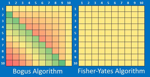
For example the row with the #2 shows the number of times over the experiments resulted in that card ending up in the position depecited by the column.
Shares shaded yellow depict expected values. Shares shaded red are results below average (peaking approx 22% below expected), and those shaded green occurring more frequently (peaking approx 30% more frequently than would be expected).
As expected, the Fisher-Yates algorithm is smooth and evenly distributed over the grid. The bogus algorithm has obvious patterns in the way the bias is distributed. With the bogus algorithm, some cards are much more likely to end up in certain positions in the final deck.
Random Number Generator
I hinted at this before, but with factorials involved in their calculations, the size permutations grows very large quite quickly. If we're not careful, they can exceed the precision of our Random Number Generator. If we're shuffling a deck of regular cards there are 52! permutations.
52! = 80,658,175,170,943,878,571,660,636,856,403,766,975,289,505,440,883,277,824,000,000,000,000 ≈ 2225.6
To be able to fully represent all possible decks arrangements, the RNG must be able to generate at least this number of distinct numbers. To correctly shuffle a deck of cards, a RNG must have a presision of at least 226 bits.
|
It is impossible for a generator with less than 226 bits of internal state to produce all the possible permutations of a 52-card deck. The RNG built into many languages can be only 32 or 64 bits in length so cannot fairly generate numbers with precision enough represent all permutations of a deck of regular cards. (Even if you have a much more precise RNG, make sure it is seeded a number of sufficient bit depth too). |
|
Summary
It's amazing to think that such a large bias could manifest from just a couple of lines of, otherwise, simple looking code.
You can find a complete list of all the articles here. Click here to receive email alerts on new articles.
© 2009-2014 DataGenetics Privacy Policy