Approximating the Sine Function

Sines and cosines are familiar to all students of trigonometry. Typically associated with right triangles, they are projections onto Cartesian x and y axes of a line sweeping around a unit circle centered on the origin.

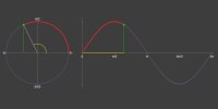
Below is an animation showing the sine function. Sines and cosines are periodic in nature and repeat after a complete revolution of the unit circle in 2π radians (360°).

There is no exact polynomial equation for a sine wave. Those familiar with Taylor’s and MacLaurin’s functions will know they can be approximated by an infinite series of polynomials.

For example, close to x=0, the value for sine can be approximated by:

That’s a lot of calculation.

These days, computer CPUs have built in trig functions and these are heavily optimized, but when I first started with coding you had to do everything yourself. In the interests of speed, often approximations were acceptable that gave results that were ”good enough” which could be calculated computationally cheaply. Typically, these approximations were used in games.

Let’s look at some ways we can approximate the sine function (and thus the cosine function, which is just the same, with a constant phase lag).

Because of the periodic nature of the sine wave, we only need to consider a small part of the continuous function (which repeats every 2π radians). With simple reflections and translations, if we can approximate just one part, we can use this to determine the sine at any value.

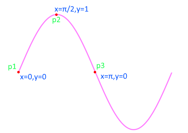
If you look at the first hump of a sine wave it looks vaguely quadratic in nature. If we were to generate this as a quadratic, how good is this polynomial approximation?

Let’s break out a little math. To generate a quadratic, we need to specify three points. We can select the two locations where the function crosses the x-axis, and the peak value: p1, p2, p3.

The generic formula for a quadratic is:

For the three points: p1, p2, p3 we can generate three equations:

Combining these simultaneous equations, we get the results that.

This gives the equation:

Which is pretty neat, just a couple of multiplications, and a subtraction, we have a quadratic approximation for sine. Pretty cool!

OK, how good is this approximation? One way to quickly see is to try and use it! Using the formula above for sin, and applying the appropriate translations/reflections to extent outside of the range 0-π and making a cosine approximation with a phase lag, we can use these approximate sine and cosine functions to regenerate the unit circle. (Use the buttons at the top to toggle rendering of each curve).

As you can see, the results are fairly good. Sure, the circle is slightly distorted, but as a first approximation it’s really not bad. If you were using these approximations in a rapidly moving game, you’d probably not notice the difference too much (though to be honest, if you needed that much speed, the old standby of usiong a pre-computed look-up table of values would be your best choice! If you had the memory; The dilemas modern programmers don't often have to be concerned about …)

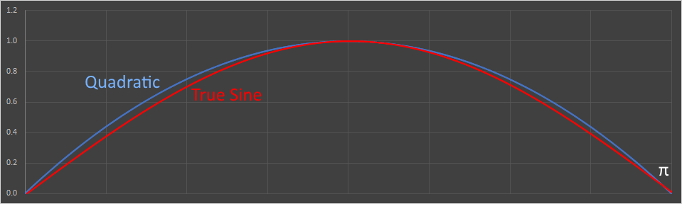
Mathematically, how good is our approximation? Let’s take a closer look. Here is a plot of the two curves over the range 0-π. You can see they are close, to a first order approximation.

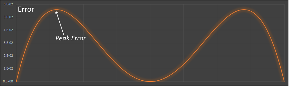
Below is a plot of their differences over the same range. The peak error is approximately 0.056 (12.2%), corresponding to around 0.47 radians (approx. 27°). This the worst the approximation gets. The error is the difference between our approximation and the true value of sin at that location. Interestingly, the quadratic approximation is always higher than the true sine.

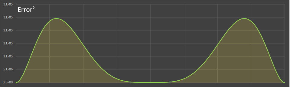
However, a better measure of “goodness” can be obtained by squaring the error (to both always make it positive and penalize large variances), and integrating over the entire range.

Here is a plot of the error squared. The smaller we can make the area under the curve the “better” our approximation is (I’m using “better” in quotes here as it’s open to interpretation what better means, depending on your need).

The approximate sine function we derived above is always larger than the true sine value.

Can we get a slightly smaller squared error if we relax our constraints? To calculate the quadratic above we applied the restriction that the curve passed through the three points: p1, p2, p3 (these were sensible constraints as we know the true sine function passes through these cardinal points). What if we removed these restrictions, and generated a quadratic with the lowest squared error?

If this resulted in a quadratic that straddled the sine function this might lower the total error even if it did not pass through the cardinal points.

Let's take a look.

Here is the formula for the error squared metric. We take the difference between the quadratic approximation and the true sine, square it, then integrate it over the range we care about.

You can expand this out and do the integration (better make a fresh pot of tea), or you can cheat and use WolframAlpha. You get this result:

We now need to determine the values for a,b,c to minimize this function.

Calculus comes to the rescue again, and we can find the turning points by calculating the partial derivatives with respect to each variable and setting these to zero.

This gives us three equations for the three unknowns:

A little bit of substution later gives the values of the three variables.

This gives the final formula for the quadratic as (I've also given the approximate decimal values for the parameters):

Here we can see how this new quadratic looks against the unit circle.

As you can see, it's a better fit and laces in and out of the true sine circle. It lowers the squared error this way (like a least squared fit), but at the expense that it's not 'true' at four cardinal points (though it is true at twice as many points as the first quadratic!)

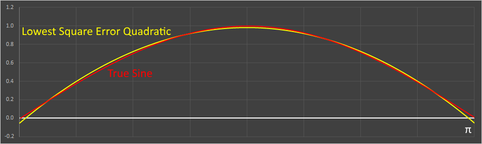
Here's our least squared error quadratic plotted next to the true sine. You can see it's much closer, and vacilates over and under the true curve to keep the error low.

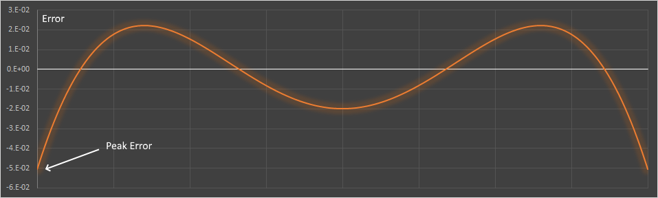
Here is the difference (error) between the the two curves. As you can see, this time, sometimes the errors are positive, and sometimes negative. The peak error occurs at zero.

And finally, here is a graph of the error².

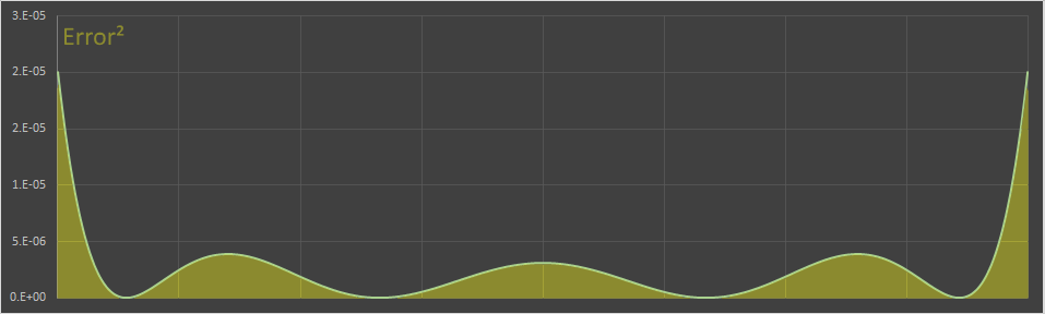
Our first quadratic had an errors squared intergral of approx 0.00404 The least squared quadratic reduces this to approx 0.000957 (a four fold improvement).

Can we do better still? Using a single quadratic, no. The least squared quadratic, by definition, minimizes the error squared integral (and we proved this with Calculus). We could get a better fit curve by increasing the order of the polynomial. Instead of using an order two polynomial, we could fit a higher order through more known points, but there's another fascinating and historical approximation created by the ratio of two quadratics. I'll explain it first, and then we'll look at a (potential) way it was discovered, because, it's so old, and there is no documentation about how it was originally derived.

Back in ancient times (c. 600-680), long before Calculus, and even when the value for Pi was not known very accurately, a seventh-century Indian mathematician called Bhaskara I derived a staggeringly simple and accurate approximation for the sine function. This formula is given in his treatise titled Mahabhaskariya. It is not known how Bhaskara I arrived at his approximation formula.

Here is his formula. It's quotient of two quadratics.

This approximation is so good that, at the scale of the graphs I'm using here, the curve is indistinguishable from the true sine curve. Below, the true sine line is shown in the red-dashed line, and the approximation in blue.

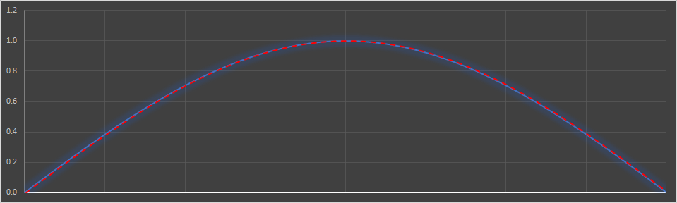
When used to plot the unit circle, at the resolution of this web page, the 'circle' produced by Bhaskara is indistinguishable from a true unit circle.

As mentioned above, there is no record about how Bhaskara derived his equation. Here is some speculation of a way that it could have been done. Hold on, we're on for a bumpy ride …

Let's go back to our first quadratic approximation:

This approximation was accurate at the cardinal points of x=0, and x=π (where the curve crosses the axis), and also at x=π/2 (the peak), but not so accurate in the middle. We know that sin(π/6)=0.5; this is sin(30°); similarly at x=5π/6, 150° the value should be 0.5 If we insert the value x=π/6 into the above equation, we get y=5/9 and not the desired value of 1/2. If we could find a way to scale the above equation to make so the value at x=π/6 was 1/2, without disturbing too much the other values, we might have a solution …

We can apply a scale factor by dividing by another function. It can't be a linear function (as this would adjust all values the same and change the end points). Let's try another quadratic …

We need the value at x=π/2 to remain the same so the value of our denominator function should be 1.0 at this point. We've also determined that the value at x=π/6 should be 1/2, but it's actually 5/9, so if we can make our denominator factor here 10/9, then (5/9)÷(10/9) = 1/2, which is what we need. For symmetry, we also want our denominator function at x=5π/6 to have a value to 10/9.

We now have three points, and can make a scaling quadratic.

(x=π/6, y=10/9)   (x=π/2, y=1)   (x=5π/6, y=10/9)

Plug these points into the generic quadratic formula gives three equations. We need to determine the three unknowns: a,b,c.

A little substition reveals these constants are:

This gives the equation for the demonimator function to be:

Inserting this into the ratio, and simplifying, gives this result.

Which happens to be Bhaskara I's equation! I have no idea if he derived it this way, but it's certainly a very cool equation. The accuracy, for such a simple function, is staggering!