Verlet Integration
In this article we’re going to look at some simple physics simulations using a technique called Verlet Integration. We’ll start with some basic concepts, build on them, and finish with a couple of fun little interactive demos: One for a piece of fabric, and the other for a rag doll stickman.
To keep the simulations simple, I’m cutting lots of corners. I fully understand these simulations are not truly faithful to the real physical world. These techniques are, however, good enough that they ‘feel’ correct and seem natural (but don’t try and launch a satellite using them!) They are also a lot of fun.
Newton's Laws

We’ll start with Newton’s Laws of motion. Newton's laws pretty much define what a forces are, and how they affect bodies. Written over 300 years ago, they laid the foundation for classical mechanics.
Paraphrasing his First Law: "An object at rest remains at rest, unless acted upon by an exterior force. An object in motion remains in motion, at a constant speed, and in the same direction, unless acted upon by an exterior force".
To the right is a particle. It's not moving. If there are no forces acting on it, it stays there. We can identify its position (in 2D) using a pair of coordinates that record its displacement from a fixed origin.
If there are no exterior forces acting on it, as per Newton's First Law, it remains where it is. What about moving objects …
Below is a simulation of a particle moving in just one dimension (click Start to animate).
The particle has no exterior forces acting upon it, so it keeps moving at constant speed (when it gets to the end, the simulation resets).
The animation happens because, like in movies, we are redrawing the scene many times a second, and each time the particle is in a slightly different position. The coordinates of the particle are updated to make it move.
If the current position of the particle is xn, what will be the value of xn+1 on the next frame of animation?
There are a couple of ways to determine this. The first way is to store a velocity of the particle. On each update (time slice), the position of the particle can be updated based on the velocity (distance traveled is the velocity multiplied by the time). This method is called the Euler method (after the famous mathematician Leonhard Euler). What this is doing is integration.
However, since we know that there are no exterior forces, and thus no acceleration (rate of change of velocity), we can say that the particle will move just the same amount in the next frame as it had in the previous frame. xn+1 = xn + (xn-xn-1) = 2xn-xn-1. There is no need to store the velocity term for the particle. (In fact there are stability advantages to not storing and using the velocity, as we will see later).
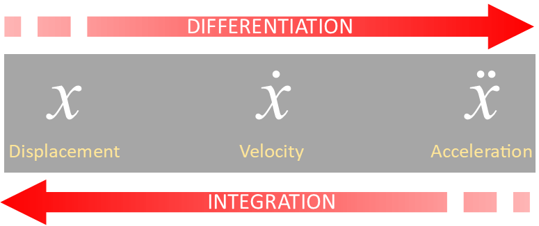
The rate of change of displacement (with respect to time) is velocity. The rate of change of velocity is acceleration. If you are familiar with Calculus, you will appreciate the rate of change of something is called differentiation (Engineers also sometimes talk about the rate of change of acceleration, giving it the term 'jerk'; it describes how an acceleration changes. It's an important concept in roller coaster design; how does the acceleration change over time in a ride*).
The inverse of differentiation is integration (hence why this technique is called Verlet integration). At the current time, we have no external forces acting on our particle (so the acceleration term is zero - no rate of change of velocity), so the velocity component is constant. Because of this, it does not matter if we use an Euler method of a Verlet method (but we'll come back to this). What we've learned is that we don't need to store the velocity of a particle; we derive it as needed.

*Just because they can, engineers have given names to higher derivatives. The rate of change of jerk, is called snap (or sometimes jounce). The rate of change of snap is called crackle, and, you guessed it … the rate of change of crackle is called pop!
Whilst these might seem a little hard to get your head around, there is a famous quote from President Nixon, "The rate of increase of inflation is going down". Inflation is the rate of change of prices (first derivative with respect to time). The rate of change of inflation is the second derivative, and the rate of how this was changing was the purpose of the quote. Prices were increasing (positive inflation), the rate of inflation was going up, but the rate about which it was going up was decreasing! Ahhhh politicians …
Ping Pong Bounce
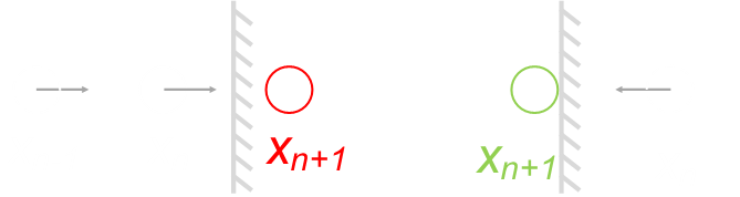
Let's constrain the particle. Rather than have it shoot off the end of the page and carry on forever, let's have it bounce backwards and forwards in the little box we've draw around it.
This is simple to achieve. What we can do is detect if the next move will place the particle beyond the end of the box. If this happens, we can place the particle exactly at the end of the box. To invert the velocity (send it back the other way), as we're not recording the velocity, in addition to updating the position, we change the value of the previous position to make pretend that's where it would have come from in order to have the velocity we need.
If we were just dealing with point particles, we could do something like this:
PX+=(PX-PX_OLD);
PX_OLD=PX;
if (PX>WIDTH)
 {
  PX=WIDTH;
  PX_OLD=PX+VX;
 }
But since the particle we're rendering has a finite radius, we need to account for this. We can also add code to bounce it at the other end. It's not perfect solution (especially if the particle is moving quickly and the previous position is just short of the wall, but it's good enough for our needs, and ensures the particle remains inside the box). Better accuracy can be obtained, if needed, by making the time step smaller; as with all things, it's a trade off. This method keeps the core loop simple, as we will see as we add more points. (every point is simply updated from its current position and its previous position).
PX+=(PX-PX_OLD);
PX_OLD=PX;
if (PX>(WIDTH-RADIUS))
 {
  PX=(WIDTH-RADIUS);
  PX_OLD=PX+VX;
 }
else if (PX<RADIUS)
 {
  PX=RADIUS;
  PX_OLD=PX+VX;
 }
Collisions and Drag
The simple ping-pong bounce simulation above will carry on indefinitely, losing no energy. We can make the simulation seem a little more 'believable' by adding the concept of non-elastic collisions and drag.
In the above simulation there are two extra options selectable. Selecting non-elastic collision results in the particle bouncing back with only 90% of the velocity it collided with the wall at. Each times it bounces it will lose 10% of it's current speed.
Selecting drag slows the particle down continuously, not just on collisions. In the above simulation, if drag is selected, after the velocity term is calculated, only 99.9% of it is applied to calculate next position (yes, yes, I know drag is more complex and is more proportional to velocity square, but read the caveat at the beginning of this article about making this a simple simulation).
You can turn either/both of the drag/elastic collisions on/off when the simulation is running.
2D
Let's apply all these principles and add a few more concepts. The above simulations were just concerned with 1D (a particle moving in the x-direction only). We can do exactly the same calculations with a y-component to make 'balls' that bounce around in a 2D box.
(Note - In this model there's no concept of surface friction; we'll add that later, so at the moment, the floor acts like a piece of ice! Also, it resets itself after a little while to stop it animating forever. Click start to get it going again!)
In this simulation, non-elastic collisions are on by default (a particle bounces back with only 90% of the velocity it collided to the wall with), and drag is on at 99.9% so that on every update, each particle travels at 99.9% of its speed on the previous frame.
There are buttons to have 1, 10, 100 or 1,000 particles bouncing about the screen, but also a new button Gravity, which applies a constant downwards force to all the particles when enabled.
This is where one of the advantages of Verlet comes in. In an Euler simulation, each particle has position components and velocity components. The force applied to each point determines the acceleration of that point, this then updates the velocity of each point, and these new velocities are used to determine the new displacements. When forces are constant, this is not an issue, but when the forces are variable, so are the accelerations, and the Euler approximations have a tendency to 'blow up' (small errors accumulate and feed forward, causing instability). This can be partially addressed by reducing the time step even more if necessary. Verlet is significantly less susceptible to blowing up.
An additional advantage of Verlet is the simple way it allows for constraints and connections between points (as we'll see below). Instead of applying velocities to points that eventually satisfy a constraints, one can simple position the point where you want it to be and let the integrator take care of things.
The gravity term can simply be applied by adding it to each of the y components of the vertices on each pass.
Adding Links
Now that we have points (vertices) bouncing about, we can connect them with links (sticks). Each link is defined by the two points at its ends.
Here's a quick demo:
You can render and see the effect of two, three, and four points connected with links (with four points, I'm connecting them either as a quadrilateral ring, or as a braced quadrilateral with an extra link between the two opposing vertices).
In this example the links are infinitely flexible and don't constrain the geometry. Updating the simulation is as simple is iterating over all the points and updating each individually. You can also turn on an off gravity.
Now let's make things a little more interesting and start to use the links to impose constraints on the points …
Constraints
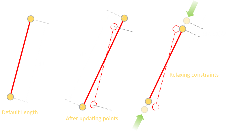
Instead of the red links being infinitely flexible, imagine they are connected with very stiff rods. The default length is defined when the geometry is created. We're going to try and keep each rod at the default length. Each time you click reset, a new random shape is generated.
To update to the next frame, the first thing we do is iterate through all the points, as before, updating them individually.
Then we iterate over the sticks. Each stick has a default length (it's length in the original geometry). We can calculate the new length of the stick, based on the new positions of the two end vertices.
There's a good chance it's not the right length! If the current length of the stick is too short, we want to push out the vertices to get it back to the correct length. If the current length of the stick is too long, we want to bring the vertices closer together.
This correction is applied by moving each of the vertices half the difference in the appropriate direction (moving each end point half of the way each to correct the error).
The pseudo code to adjust the position of the end vertices is something like this:
  dx=PX[vertex1]-PX[vertex2];
  dy=PY[vertex1]-PY[vertex2];
  d2=sqrt((dx*dx)+(dy*dy));
  diff=d2-d1;
  percent=(diff/d2)/2;
  offx=dx*percent;
  offy=dy*percent;

  PX[vertex2]+=offx;
  PX[vertex1]-=offx;
  PY[vertex2]+=offy;
  PY[vertex1]-=offy;
Using Pythagoras, the new length of the stick is calculated. The difference from the original length is calculated as a percentage (this can be negative if the new length is shorter, but the sign takes care of all the math). This difference is divided by two as we want to apply half the update to each vertex. Pro-rata, this percentage is applied to the deltas in the x and y components, then these offsets are appropriately added and subtracted from the end vertices.
All the sticks are looped over, and each gets a chance to apply its constraint and adjust the geometry, then the mesh is rendered. It might sound like chaos, and a lot of push-me, then pull-you, but as you can see, it works pretty darn well for such a simple piece of code!
When I first started this, I was convinced that all these constraints would result in n-sets of simultaneous equations that would need resolving (which would be slow), but as you can, simple selfishly moving the points based on each constraint in isolation seems to do a fairly good opening job. I also thought it might be important of the 'order' in which the constraints are applied (as each time a stick's constraint is applied, it adjusts the position of the two vertices, which could be used by other sticks), but as it happens, it all comes out in the wash!
Here's the core loop:
if (RUNNING) {
updatepoints();
updatesticks();
render();
}
Spend a few minutes playing with this, reseting with random shapes, and you might start to see a couple of issues. We'll address these issues in the next iteration of the code …
Issues
After playing with the above animation for a while, you might have encountered the first issue (especially if you have gravity on, and on the first drop of the shape), and this is that sometimes points get drawn outside of the boundary!
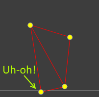
What's going on here? I thought we moved each of the vertices inside the box after they were updated?
We did, but when we update the sticks, the constraints have freedom to move the vertices again. It could happen that applying the constraints moves the vertices outside the bounding box.
Thankfully, this is a really simple issue to fix. We take the code that checks the position of the points and move this into it's own function, and apply it after all the coordinates are updated.
Only after everyone who wants to has updated the points, we constrain them to be inside the box, then render.
if (RUNNING) {
updatepoints();
updatesticks();
constrainpoints();
renderpoints();
}
Again, this highlights one of the wonderful advantages of Verlet integration; we can move any point where ever we want, applying whatever constraints we wish. Because each point remembers it's previous position, and only these things are used to determine the future positions we don't need to worry about what trying to calculate what the velocities would have been to make the moves! Simple!

The second issue is a little more subtle.
If you play with the above simulation for a little while you will see that the shapes seems to wobble around (especially just after a collision), like a jelly on a plate.
This is understandable, as when the sticks are being updated there is a juggling; some want to push vertices, some pull them. Often there are conflicts which resolve themselves as the points shuffle and settle.
The fact that things settle down is the key to how to solve this. What we can do is update the sticks (and constrain the points inside the box), multiple times until things settle down. We give chance for all the geometry to settle down and shuffle before rendering.
if (RUNNING) {
updatepoints();
  for (int i=0;i>ITT;i++) {
  updatesticks();
  constrainpoints();
  }
renderpoints();
}
We must be careful to only update the points once, otherwise the forces would be applied multiple times. Inside the loop the sticks apply their constraints and move the points around, pushing and pulling as necessary. Finally the points are rendered.
The exact number of iterations needed depends on the geometry, parameters, time slice … so it's one of those things that you might want to experiment with to find what works 'well enough' for your needs. As with all things, it's a trade off. The more you iterate, the more the constraints relax against each other, but the more processing is needed. Using my simple example meshes, just a couple of iterations seems to work fine.
Below I've implemented a way to experiment with this. The simulation allows you to adjust the number iterations of the relax constraint loop. When at one, it's the same as before, and the shapes wobble as they they bounce. By the time the loop is at four, things are pretty rigid.
Use the bottom row of buttons to specify how many relax constraints is looped.
Further down the rabbit hole
From above you can see that the braced quadrilateral keeps its shape as the middle brace turns it into a triangular mesh.
Sticks don't have to rendered even though these are used in the calculation! An additional attribute can be added to make them invisible and not rendered. In the below simulation I've taken it a stage further. Below is a random braced quadrilateral; none of the sticks are rendered, and I've drawn a polygon around the outside vertices.
In this model I've applied a crude friction system which constrains the x-coordinates if the y-coordinate reaches the bottom. You can turn this on or off using the button.
An additional thing added to this simulation is the ability to move the quadrilateral. You can drag any corner of the quadrilateral to move it about the screen (go in, try it!)
Again, this is easy to achieve with Verlet because all we do when dragging the vertex is updating the new coordinates for the point to reflect where it is being dragged to. The previous coordinate points are stored, and this takes case of all the geometry and movement needed on the next cycle. No need to worry about velocity!
Different constraints
Here are a couple more examples of applying constraints. In these examples, we're making vertices that are fixed. In the core loop, if a vertex is marked as fixed, it's coordinates are not updated.
In both animations, the vertex at the top of the chain is fixed. If a vertex is marked as fixed, it is not possible to be moved (by either the updatepoints() function or updatesticks() functions. It's current and past position coordinates remain fixed. (Strictly speaking we could optimize the updatesticks() function so in that, if one end is constrained, the other the moves the entire delta, instead of half, but as we loop through the relax contraints loop a few times, this seems to take care of itself pretty quickly.
In the animation on the left, you can drag any vertex of the quadrilateral around (then let go). In the animation on the right you can move the anchor point at the top of the chain around by dragging it. It's still a fixed vertex in the animation, but you can move where this fixed position is (like a ball on a chain).
Each time either is reset, a random quadrilateral is attached to a multi-link chain.
(If you are a little aggressive, depending on the geometry of the random shape, if you swing the pendulum on the right hard into a wall, you might find it 'pop' into a different, canonical, shape that also satisfies the geometry constraints of the distances between each of the vertices).
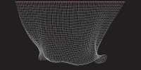
Fabric Simulation
Putting all these ideas together we can make a really fun fabric simulation.
We'll make a slight modification to the constraint update function. In the above systems, the sticks are rigid, symmetrically, in both tension and compression; their only goal is to try and keep the geometry the same as originally defined (pushing and pulling as needed).
We know, in real life, that, whilst you can pull a piece of string you can't push one!
To make this change we only attempt to update constraints if the separation is greater than the default length. If the separation is less than the original geometry, we don't update. In this way, the sticks behave like one-way constraints (springs), active only in tension, not compression. They behave more like pieces of string instead of wood.
In the simulation below is created a mesh of particles, each connected to it's nearest neighbour forming a fishnet curtain. The top nodes are fixed near the top of the box. When the simulation is started, all the coordinates are setup at the top (+/- some small random deviation each time, to give it a bit of swish), and the curtain drops down in a pleasing way!
Finally, because the whole idea of this simulation is to see the intermediate results and the 'conflicts' of the constraints, I only call the constrain function once (not many times as we did with the rigid shapes).
Using the mouse/finger you can brush over the mesh to displace it. What this does is try to move all the vertices in a defined radius from the pointer away from it. This allows you to ripple the fabric!
But wait, the fun is only just beginning …
If you are on a slow computer, or just want a shorter curtain, there is an option to use either a Full or Half sheet of fabric.
You can also specify the number of attachment points at the top of the fabric. By default this is set to 'Full', where every top node is connected. Other options include 'Partial', 'Sparse', or just 'Corners' and these buttons determine the number of top row vertices that are classified as fixed.
Now onto some really fun things: We can selectively remove some links on the mesh. If you are reading this on a PC, and have a right mouse button, you can use your right mouse to cut any of the links on the mesh. If you don't have a right mouse button, or you are on a tablet or mobile, you can use the bottom left button to toggle between 'Move' and 'Cut'. The default state is move, which moves the mesh around. In cut mode, clicking on the mesh destroys link with a midpoint closest to the click (within a reasonable threshold). You can experiment with tearing and making holes in the fishnet.
But it gets better! By default the rip resistance is set to 'No tear' meaning any link can take any infinite amount of tension. To more realistically model fabric, we can specify a maximum value of tension, above which, a link will break. With this you can experiment with make holes in the fabric, then turning to move mode and blowing over the sheet seeing if you can get the holes to propagate. Take care! With 'Weak' tear resistance, the act of simply dropping the curtain can be enough to cause the fabric to rip on reset (change it to higher resistance before reset, let it stabilize, then change the rip resistance).
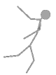
Stick Man
Now onto our final simulation. That of a rag doll stick man.
In homage to Sherlock Holmes, and The Adventure of the Dancing Men, here, using the principles of Verlet integration, is a simple rag-doll man simulation where you can throw a stickman around the screen!
You can turn on or off gravity to experiment with him either 'floating' in space or with the brutal effect of gravity pulling him down. You can also turn on or off friction to decide if the floor behaves like a sheet of ice.
Probably the most fun, however, is your ability to grab the man by one of his joints and throw him against a wall, or launch him, or simply move him slowly and drag him, drooping, around the box. Poor Mr Stickman.
With care, you can grab him by the foot, knee, pelvis, mid-back, shoulder, elbows, hands, or head.
How does it work?
The animation uses all the concepts we've applied so far, and adds just a couple of extra (invisible) springs.
It also adds the concept of a stiffness property to each of the links.
First I created a vertices for all the joints, then connected these, as appropriate, with sticks to make the man, and added a head!
Each of these links is given a stiffnesss coefficient of 1. When the next frame is calculated and resolve constraints is called, the delta between the current length and the desired length is calculated (then halved), and applied to each end vertex. This new change applies a coefficient that modifies how much of this error correction is applied. All the body links are given the coefficient of 1.0 so that on every update, all of the required delta is applied. By giving lower values. we're 'damping' the correction that is applied; we know there's an error, it's just that we're not going to apply it all straight away. A value of 0.5, for instance, would mean that we only move the vertices half of what is needed to put them back to a mean position.
With a value of 1.0 these links should behave like rigid sticks and be pretty close to the default length at all times (only varying slightly based on conflicting constraints during the resolution process).
Next I added some additional (invisible) links to represent springs. For these I experimented with a variety of stiffness coefficients ranging from 0.1-0.2 (meaning only 10%-20% of the required correction is applied on each frame).
I also experimented with keeping certain joints under tension (sort of like pre-stressed concrete) by adjusting default length of the hidden springs. When the man is created, using Pythagoras, I know the distance between the vertices. However, for the spring link, the value I enter in for the default link length is 95% of this. This creates a constant force trying to straighten the link, even though it might be constrained by other geometry.
I experimented with putting these hidden springs between one foot and the opposite knee (to spread the legs out), one between the elbows, one from each hand to the shoulder, and also one from the hip to the head to stop him going spineless. I'm not claiming these are great choices, not model how a real stickman might behave if thrown around a room, but hey, it gives pleasing results!