Heavy Hitters Algorithm

Imagine there is a huge bucket, and this bucket is full of balls of various colours. You don’t know the total number of balls in the bucket, and you also don’t know the number of distinct colours the balls could be. Your task is to determine what the most popular coloured ball is in the bucket (the modal colour).

You proceed by taking a ball out of the bucket, noting it’s colour, acting on this information, then taking the next, then the next, until there are no more balls in the bucket. What is your strategy for finding the most common colour?

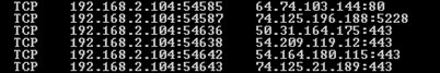
This is a common problem in computer science. If, instead of this being about balls in a bucket, imagine they were log files for some service which you were reading sequentially. For instance, they could be logs of search terms and you are trying to find the most commonly searched query. Maybe these are error logs files and you are trying to find the most common error, or possibly IP addresses of incoming requests and you want to know who is using your service this most. You might want to know about volatile trading from a stream of stock trade data. Twitter wants to know what the top trending hashtags are, and Amazon might want to know what it’s best-selling products are …

This type of search is often called the search for Heavy Hitters. (Or the search for elephants, or icebergs). It’s a very well known problem and has been studied pretty much for as long as computers have been around.

As a first blush, it seems we should be able to do this in one pass (which is the Holy Grail for algorithms of this type, and is something that can be applied continuously on a stream). We could sequentially work our way through the stream, hash each input, and keep a frequency count for each hash. The hash with the highest count is the most popular item. Done!

This would be a fine solution if the number of distinct items in the dataset were small (for example if there were only a dozen possible colours of ball in the bucket), but at scale, this solution falls down. If, instead of colours, these were IP addresses, there could, theoretically, be billions of distinct inputs, and you’d be memory bound. Also, because you don’t know the distribution of the traffic (it’s essentially random), you can’t keep a rolling window of the ‘current top n’ items as there is no guarantee that the most popular item does not start popular, then get overtaken by a spike of other traffic (and thus be dropped from the cache of current ‘winners’), and thus get lost when it gets a second wind later in the stream.

If we add the restriction that the data set has a majority element (an element value that is repeated more the n/2 times in a set of size n), there is a clever algorithm attributed to Robert S Boyer, and J Strother Moore, called the Boyer-Moore Majority Vote Algorithm, which allows determination of this element without extra storage being needed.

Before looking at the Boyer-Moore algorithm (and some extensions), it’s worth examining just how important these kind of algorithms are, and the ability to determine values from a stream, or incrementally. I’ve written a little about this before in this article about incremental means and variance.

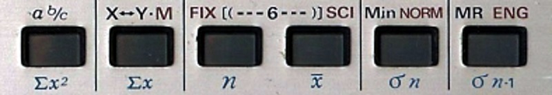
Imagine you have a stream of numbers and want to calculate the mean of these numbers. It’s easy to see that you don’t need to keep track of all the individual numbers you have seen. All you need is to keep a running total of the sum of the input, and the number of items seen to calculate the mean. With a little extra math (Storing the sum of the squares of the input), it’s possible to determine the variance (and thus Standard Deviation) of the set without having to store the individual numbers. This is how your pocket calculator statistics functions work.

(Practically, however, there could be issues with this approach to means/variance at scale because of precision issues, and potential overflows, so with a little math it’s possible to come up with incremental formulas for mean and variance that don’t rely on having to keep track of the sum and sum of squares, but instead derive their answer based on the last results for these values, and how these are changed by the current sample. The derivation of these incremental formulae is given here).

Interestingly, returning to the heavy hitters, if we apply the majority element restriction to a stream of numbers we can see that the search for the Modal element reduces down to finding the Median (Because, if there is a Majority element, by definition, it has to span the Median). If our stream were sorted, and there was a guarantee of a majority element, we could find the most popular element by simply taking the middle element!

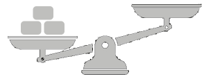
To see how Boyer-Moore works it’s first helpful to think about pairing off, and casting out, distinct pairs of elements.

Returning to our bucket of containing n balls. Let’s imagine that there is a majority element, and this is a red ball with |red|>n/2.

As a thought experiment, imagine if we pulled balls out of the bucket in distinct pairs, then threw these pairs of balls away. There are only two possible kinds sets we can pull the pairs of balls out as. The first is a red ball and some other colour, and the second is two distinct colours that are not red:

In either case, the concentration of red balls left in the bucket increases.

When we throw away a pair of non-red balls (for instance a green ball and a white ball), we’re reducing the number of balls left in the bucket, but the number of red balls stays the same. If we pick up a red ball and something else, yes, we’re removing a red ball and reducing the number left, but since there are more than n/2 balls that are red, even if we happened to pick a red ball with every pair, there would still be at least one red ball left after we can’t pair up any more distinct balls.

Eventually we’ll only be left with red ball(s) in the bucket; unable to distinctly pair off anything else, and proving that red is the majority element.

To be honest, we don’t care about what the colours of the balls are if they are not the majority element, and this is the heart of the Boyer-Moores majority algorithm (shown below). What the algorithm does is walk through the stream keeping track of a candidate item for the majority element. Every element that comes along that confirms this candidate, increases the belief and increments a counter. Every element that comes along that refutes the current candidate decrements the counter on this candidate (analogous to casting out pairs). We only need to keep track of the current candidate, which may change many times through the pass, however, as the frequency count is a conservative field, it does not matter that path to get there, the result will always be the same.

If your favourite soccer team wins a game with a score of 4–3, it does not matter if your team score all four of their goals first, then the opponents clawed back three, or if the opponents scored all their three goals first, then you did, or if the lead vacillated between your team and the opponents and the lead changed multiple times through the game. At the end of the day, the goal difference is still the same, no matter what order the goals were scored in. For more interesting consequences of this, check out this article about Bertrand’s Ballot.

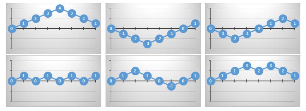
It’s interesting to see how the lead might change (what the current candidate happens to be in Boyer-Moores), but at the end of the day, the only thing that matters is what the final score is.

Here's the code for the Boyer-Moore majority algorithm. It's simple and elegant.

for i = 1 to n
 if (count==0) {candidate=A[i]; count=1;}
 else if (A[i]==candidate) {count++;}
 else {count--;}
next

Items are read from the stream, one by one. If there is no current candidate (either at the start of the algorithm, or because the count has been decremented to zero), then the current element is selected as the candidate and its count set to one.

If there is already a candidate, and the current element matches this, then the count is incremented. We're getting reinforcement that the current candidate is the modal item.

Finally, if the current element does not match, we decrement the count (this is like casting out pairs).

Once we've read the entire stream the finished candidate will hold the majority element.

NOTE - Even though the current candidate shows what the majority element is, it does not, show what the frequency of this element is. In order to do this, a second pass has to be made through the list (knowing now what the majority element is), and counting, absolutely, the elements that match (it is not possible for a sublinear-space algorithm to determine whether there exists a majority element in a single pass through the input).

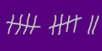
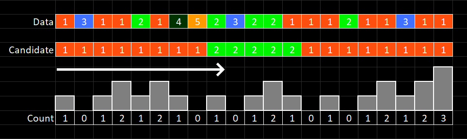
Here's a sample walkthrough of the algorithm. The stream is shown moving left to right, and the individial elements shown in the top row. The second row is the current candidate, and the third row the count for this candidate.

Interestingly, the Boyer-Moore algorithm can still be applied even if it is not known that there is definetly a majority element. At the end of the first pass, the the alogrithm tells you that, if there were a majority element, that this what it would be. It does not tell you there is a majority element. This can be achieved on the second pass. Now that a candidate is known, the second pass can count all those that match that candidate, and if this count is greater than n/2 then you know it's a majoity element.

*Ten Apples up on top – Dr Seuss

Interestingly, the simple majority Boyer-Moore algorithm can be enhanced to determine, not just the majority element candidate, but the candidates in the stream that have a frequeny of at least n/k. It does this be keeping a list of the k-1 potential candidates and their running counts. As above, just because an element appears in the output, it does not guarantee, this element occurs with frequency > n/k, just that it is a candidate. As before, a second pass is required to confirm each candidate, and the actual frequency for that element. This has potential to produce a list of top 'hot' items.

This variant of the heavy hitters is sometimes given the name of the Misra-Gries algorithm. It works in a very similar way, and the easiest way to think about it is to consider, not just casting out pairs (as we did with Boyer-Moore), but in this case casting out distinct sets of k-1 elements at a time.

Instead of keeping a single counter and item from the input, the Misra-Gries alogithm stores k −1 (item,counter) pairs. The natural generalization of majority is to compare each new item against the candidates, and increment the corresponding counter if it is amongst them. Else, if there is some counter with count zero, it is allocated to the new item, and the counter set to 1. If all k − 1 counters are allocated to distinct items, then all are decremented by 1.

The algorithm can be sumarized as this.

For each new element:

• If the item is already in the candidate list, increment the count for this candidate.
• Else if there are less the k-1 items in candidate list, add this to candidate list with a count of 1.
• Otherwise, decrement the count of every item in candidate list by 1.
• After this decrement, if any counter==0 then remove it from the candidate list.

This is a very neat algorithm, but remenber the output is only a candidate list of potential elements that occcur with frequency great than n/k. As second pass is needed to confirm and determine the exact frequency. Also, related to this, if the most frequent element has a count of less than n/k, there is no guarantee that it will appear in the solution set, even though it has the highest frequency.