
Sampling from non-symmetric discrete outcomes
This is going to be a long article, which ends in a really neat algorithm. We’re going to meander around, so grab a cup of tea and stick around.
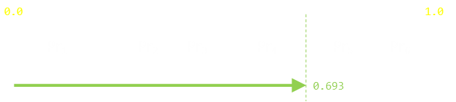
We’ll start with a trivial problem: You have a random number generator (that generates floating point numbers of sufficient precision), and want to simulate the flipping of a (fair) coin.
A coin flip has two outcomes; heads and tails and, on a fair coin, each outcome is equally likely. If our random number generator generated numbers in the range [0,1] then something along the following lines would be perfect:
Function FlipFairCoin() {
if (random() < 0.5)
return (“Heads”);
else return (“Tails”);
}
A way to think about this is in which box of the diagram below that the random number points to.
Biased Coin
What if we wanted to simulate a biased coin (one that is more likely to land on one side than another)? Again, this is trivial to code. Instead of using 0.5 as the threshold, we can pass in an argument representing how biased we want to coin to be.
Function FlipBiasedCoin(float bias) {
if (random() < bias)
return (“Heads”);
else return (“Tails”);
}
For instance, if we called the above function with FlipBiasedCoin(0.7) we would get results that, on average, were 70% heads. So far so good.
n-sided die
Now let’s graduate to a n-sided fair die. Now we want a function to return the result [1,n]. Something like the following will work just fine.
Function RollFairDie(integer n) {
return int(random() * n) + 1;
}
As the boxes are all the same size, taking the floor of [0,1] multiplied by the number of values will give an integer [0,n-1], to which we can add one to move offset off zero.
Biased n-sided die
Now things start to get interesting. What happens if we want to model a biased n-sided die?
Let’s imagine we have a set of probabilities representing the weights that we want each side to be come up:
Pr1, Pr2, Pr3, … Prn-1, Prn
How would you write code to do this? Can you see the issue?
Well, we could write code something like this (I’m not suggesting you would write it like this, but I’m making a point). The issue is that there are arbitrary boundaries between adjacent regions, and differences are cumulative as you move along.
Function RollBiasedDie() {
r=random();
if (r < pr1) return 1; break;
elseif (r < (pr1+pr2) ) return 2; break;
elseif (r < (pr1+pr2+pr3) ) return 3; break;
…
}
OK, this is a little silly, but even using a loop, you’d have to do a lot of tests! There has to be a better way. In fact there are quite a few different ways. Let’s take a look at a few simple ones, and their limitations, on the way to our ultimate (elegant) solution.
I’ll give these the names:
- Cumulative Probability
- Sultans Wife
- Lowest Common Multiple
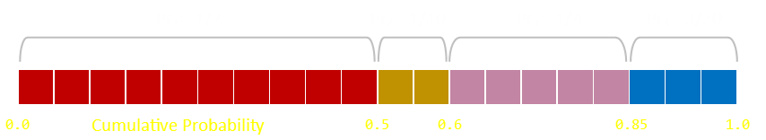
Cumulative Probability
Let's imagine the following data as an example:
Pr1=1/2, Pr2=1/10, Pr3=1/4, Pr4=3/20
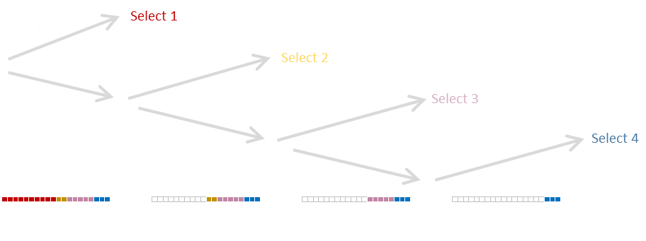
We can pass through the data once, and pre-compute an array of the cumulative probabilities. Then, when we need to find which region to select from the random number, we can scan through the cumulative probability array to find the region (value) that the hosts this number.
If there are more than a couple of distinct values to examine we can use our old friend, the binary search, to optimize this approach. Rather the ploughing through the cumulative probability array in order, we can start at the midpoint and search higher/lower, recursively, until we get to our solution.
Using this approach, we can pre-compute the cummulative array in one pass, and search/generate our numbers with log n comparisons.
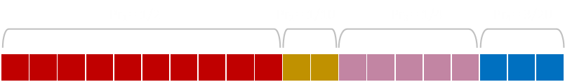
Sultans Wife
This approach takes a little more thinking, but generates just as valid a solution. It's vaguely related to the Sultan's Wife puzzle. Rather than roll just one die, we roll a die for every possible branch, and continue until we get a hit (or get to the end).
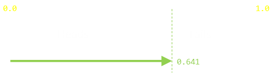
We know, in our example, that Pr1=1/2, so we have a 0.5 chance of selecting this first value. So, using our biased coin function, we roll a die (in this case with probability 0.5), to see if we get a hit. If we do, we terminate there.
If we do not select the first value, we carry on and see if the we get lucky on the second value. However, we do not use Pr=1/10. For this coin flip, our solution space is now smaller, (we've rejected half the space by not selecting the first branch). We need to normalize (scale) the remaining space by (1-Pr1), so the biased coin flip to test for the second value is run with Pr=1/5.
(Another way to think about this is we have a 50:50 chance of selecting the first value, shown in red. If we don't match this, we can throw this part away, and we have a self-similar problem, now with only three values, but we have the scale the probabilities appropriately because the length of this smaller bar is now less than 1.0)
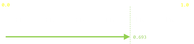
If the second value does not hit we need to scale the remaining bar by (1-Pr1-Pr2)=0.6, so the test for the third value would be a biased coin of 1/4 ÷ 4/10 = Pr = 5/8.
Generally, after flipping c coins, the remaing 'bar' left is the 1-(sum of all those rejected to date).

This algorithm does not require any pre-computed initialization steps, but the generation phase is heavily dependant on the probabilities. If you know your probabilities are going to be highly skewed (maybe some of them even zero), you might be able to do some optimisation by lightly sorting them first so that the most likely probabalities get tested first.
Lowest Common Multiple
If you have a limited variance of probabilities, and the probabilities have a lot of common factors, you can trade memory for a boost in generation performance.
As an example, using the same data as above, an array can be created, in this case with length 20 (the lowest common multiple of of the denominators of the fractions), with the corresponding desired result stored in the appropriate index.
We have now re-mapped the problem from a four sided biased die to a twenty sided fair dice roll. We know we can roll a fair die in one call so generation will be very quick.
Of course, the problem is this solution takes excess memory to store this mapping. If the probabilities have poor common factors (for instance, with just two probabilities of 1/999, and the other 1/1001, that's already 999,999 buckets needed!) Also, typically, the probabilities will be floating point numbers and not something easily factorised.
Advertisement:
Applications
Just before moving on to describe the elegant solution promised at the start of this article, it's worth taking a few minutes to consider some of the varied (useful) applications of discrete sampling with values of distinct and varied probabilities. In no particular order:
- Imagine you are streaming music and want to play a variety of songs, 'shuffled', randomly, but weighted. Every song in your library must have a chance of being played, but you want to make some songs more popular than others (because you like them more). You can apply a weight (probability) to each song, proportional to your taste of that track. Then, using the algorithm we're about to describe, you can randomly select the next track based on these preferences. If your tastes change with low frequency, you can regenerate the probability tables only when needed (taking the computing time hit for that then), because, as we will see, the generation of the random element, once the tables have been generated, is very fast.
- Related to the above you could use play data to to adjust a most recently played probability table so that songs that you've not heard in a while have a higher chance of getting airtime, whilst those just heard have a less likely (but still small random) chance of being heard again.
- If you are writing a simple load balancer, it might be your responsibility to farm out tasks to a hierarchy of slaves you control. Incoming tasks might have a random of set of variances of processing time, so you want to distribute them at random to your farm, but some machines might be able to handle more load than others. You could weight the probabilities of which machine gets the next incoming task based on the probability proportional to the processing throughput of that machine.
- There's a huge collection of applications given the generic name of Multi-Armed Bandits (for more background, read the link indicated), but as an example, imagine your are responsible for displaying adverts or some other kind of creative content on your company web page. Clearly you want to display the content that performs the best, but how do you know what is the best? If you have ten possible pieces of potential creatives to display, which do you show? Initially you don't know how each performs. If you put them all up symmetrically you are, ultimately, wasting eyeballs displaying poor performing product. A better strategy is to, initially, have them all up equaly random, but monitor their performances. As you gather data, the rich get richer, and the better performing adverts get higher weightings so that they are more likely to be displayed in the future. The poorer performing creatives still get a look in (though with reduced frequency), so that if the tide changes, the system dynamically balances, and an advert can get back into favour again.
- Maybe you are experimenting with trying to find the best price a sell a product, or conducting a drug trial with a variety of products, or attempting to find a investment portfolio mix …
 Image: Thomas Hawk
Alias Algorithm
Ok, here we go with the neat algorithm. We'll return to the example data we used before:
Pr1=1/2, Pr2=1/10, Pr3=1/4, Pr4=3/20
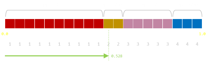
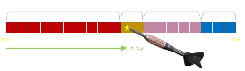
Generating a random number is like throwing a dart into the number line a random distance in the range [0,1]. Whichever region it lands in is the value we want. The size of each region is proportional to each probability.
What we can do is rearrange the line; chop it, and then stack the individual blocks a different way. If we give each line a constant 'width', we can change the lines into areas. We can then continue with our 'dart throw' mind experiment. The areas of the regions stays the same so, if we hit one of the coloured regions, we are proportional to their sizes and thus their probabilities. The only issue is if we hit the gray area which is outside of the coloured bars. If this happens, it can be solved with just a redo (throwing the dart again).
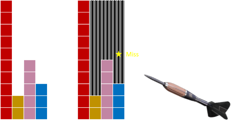
Our aim should be to minimize the the amount of gray space on the board (reduce the number of re-throws). At the moment, the 'height' of our rectangular board is the height of the greatest probability. With some thought we can see that we can eliminate the 'miss' regions by carving up some of the taller bars, breaking them into pieces and inserting them into gaps. The overall area of the coloured bars stays the same, as does their relative sizes, so this does not adjust the relative probabilities. Now, as our board has complete coverage, there are no holes, and no chances to miss!
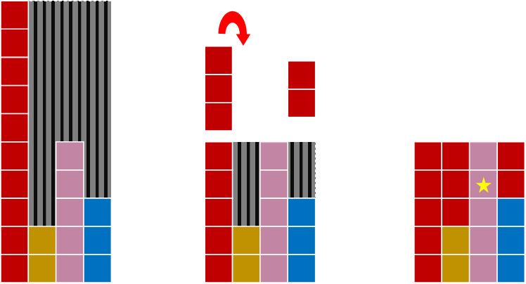
Now, to calculate the value will get, we select a column at random (fairly), then randomly select the region in that vertical column propoprtional to just the data in that column.
Here is the clever part: IF we can ensure that there are only ever two possibly values in any vertical column, then this second randomly selection is just a biased coin flip between two values (which we can trivially do). With the correct rearrangement (which we can pre-process), we've reduced the entire problem down to just a fair n-sided die roll and a biased coin flip!
We've reduced the entire problem down to just a fair n-sided die roll and a biased coin flip!
This is the alias algorithm.
Now, all we have to do is ensure that we have a mechanism so that we only ever get (at most) two distinct values in any vertical column (if we re-arrange the grid so that there is more than two in any column, we can't do the biased coin flip and we've remapped the problem to just a canonical form of the original problem of having to sample from a plurality of distinct values).
We need to ensure there are, at most, two distinct values in any column
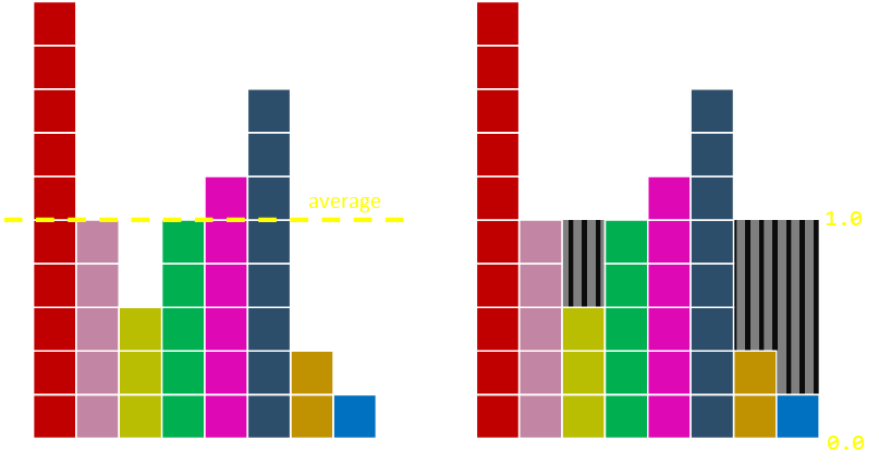
If we adjust the height of our board to the average height of the probabilities we get a nice result. The number of columns is the number of distinct values to select from, and we can then scale the vertical axis so that the average corresponds to 1.0
But how do we even know that it's possible to cut the original rectangles apart in a way that allows each column to contain at most two different probabilities? This does not seem immediately obvious, but amazingly it's always possible to do this. Moreover, not only can we cut the rectangles into pieces such that each column contains at most two different rectangles, but we can do so in a way where one of the rectangles in each column is the rectangle initially placed in that column!
Covering the second part first, you can see that, as we are cutting off the tops of some rectangles and using this to fill the throughs, we are never removing all of the first rectangular block. As we are never removing all the rectangle, at least some of the base remains, and we started off with a distinct colour in each column. The reason for the name of the algorithm as the 'alias' algorithm is that each column has a (potential) alias; and only one. We select our initial column using our fair n-sided die. There is one column for each colour, so we first decide, fairly, which of the colours we get. Then we flip a biased coin to see if we keep this selection or flip it to the alias value for this colour. The result of our pre-processing is just two arrays. The first is the list of the alias colour for each column, and the second is the probability, for that column, that we'll flip to that alias colour. (Potentially there can be no alias value, and a column can be all one colour; this is fine).
You can convince yourself of the first part by induction. Imagine there ia a grid that almost perfect with just two outstanding anomilies; one peak, and one trough. The piece we chop off the mountain has to fit into the valley as we scaled the board based on the average values. We know that the minimum of all the scaled probabilities must be no greater than the average and that the maximum of all the scaled probabilities must be no less than the average, so when we first start off there always must be at least one element at most one, and one element at least one. We can pair these elements together. But what about once we've removed these two? Well, when we do this, we end up removing one probability from the total and decreasing the total sum of the scaled probabilities by one. This does not change the average (since the average scaled probability is one). We can then repeat this
procedure over and over again until eventually we've paired up all the elements.
Using these principles, we have the basics of a simple remapping algorithm:
While not finished
Find a column (i) with Pr > 1
Find a column (j) with Pr < 1
Remove sufficient from (i) to make (j) = 1
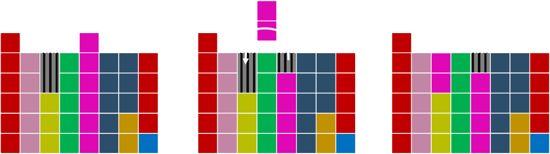
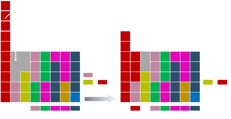
Each pass of the loop creates one column that is 1.0 so the loop will always terminate. Let's see this in action. In the data below we select the red colum as the hill column and the light blue as the through. We take sufficient off the red to fill in the void above the blue column. In this case, the red column is still above average. This is OK.
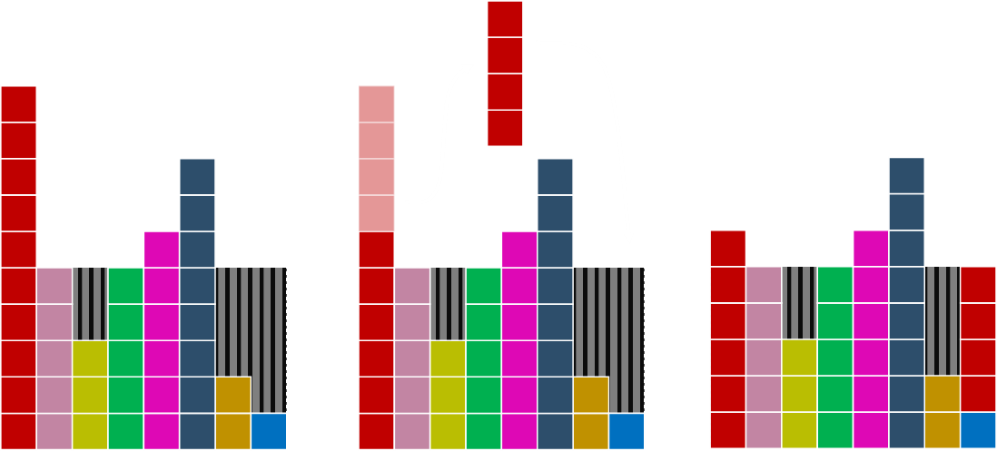
Next pass we'll select the dark blue as the hill. It does not matter which we chose; we could have selected the red, and it would still work out. As you can see from this, it means that there can be many different (equalyy valid) final solutions. In this case, after we move over the dark blue blocks, we've made both columns 1.0, reducing the number of unbalanced columns.
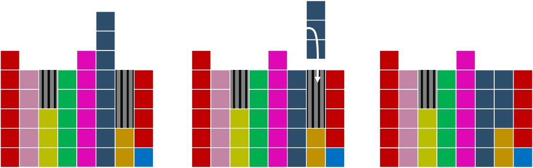
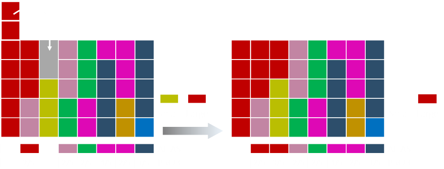
Next we'll select the magenta column as the peak, and the light green as the destination. In this case, moving sufficient magenta over to fill the void results in a new valley being created as we need to move two over. Not a problem …
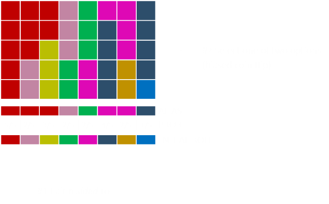
Finally, the last hole is matched up.
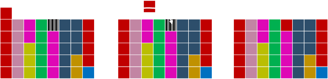
And we have our solution! Each column has the same starting value at the bottom, and each column has, at most, two different colours!
Vose Algorithm
If you end up coding the above algorithm you will see that you have to scan the column heights each pass looking for a peak and a trough to use. An optimisation could be to sort the heights first to speed up searching, but there is a varient of the algorithm, often called the Vose method (after it's inventor, Michael Vose), that balances the colums a different way and makes it more efficient.
The concept of Vose's algorithm is to maintain two lists; one containing the elements whose height are less than one (small) and one containing the elements whose height is greater than one (large). The algorithm repeatedly pairs the first elements of each list. On each iteration, an element is consumed from the "small" list (and potentially moving the remainder of the element from the "large" list into the "small" list).
(There are some other, subtle, modifications designed to make the algorithm numerically stable, especially when dealing with floating point numbers and rounding/scaling issues around whether something is just above, or just below, one. A combination of these things can end up putting too many items in the small list, and then the large list is prematurely empty). The final algorithm is below. The modification terminates then main loop when either of the lists becomes empty, and then clean-up loops by making any yet unallocated to precisely 1.0 after the main loop
On each pass of the main loop, the top elements of the small and large lists are paired, and sufficient removed from the large column to complete small one (the balancing going to back resulting in the donor column to either the large or small list).
INITIALISATION:
Create two arrays ALIAS and PROB of size n
Create two lists SMALL and LARGE
Scale each Pr by n
For each Pr
if Pr < 1.0 add to SMALL otherwise add to LARGE
Whilst SMALL and LARGE are not empty:
Remove top element from SMALL (s)
Remove top element from LARGE (l)
Set PROB[s]=Pr[s]
Set ALIAS[s]=l
Set Pr[l]=Pr[l]-(1-Pr[s]) // use (Pr[l]+Pr[s])-1 for numeric stability
if Pr[l]<1 add (l) to SMALL else add (l) to LARGE
Whilst LARGE is not empty:
Remove element (l) and set Pr[l]=1.0
Whilst SMALL is not empty: (only happen with numeric instability)
Remove element (s) and set it to Pr[s]=1.0
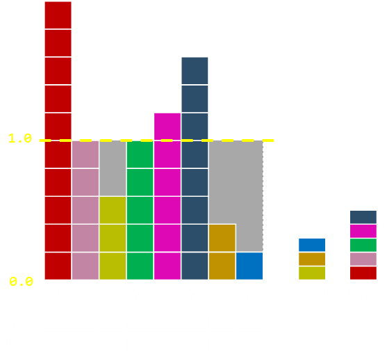
Everything works better with pictures. Let's run through the last example with this new algorithm. To the right is shown the two lists; each column is in either the small list, if shorter than the average, or in the large list, if equal to or above the average. Notice on each iteration that the base of the column remains it's initial colour and that, on each iteration, at least one complete column is created.
In this example we have eight samples, the initial probabilities are:
Pr1=1/4, Pr2=1/8, Pr3=3/40, Pr4=1/8, Pr5=3/20, Pr6=1/5, Pr7=1/20, Pr8=1/40
The first part of the algorithm is to scale everything so that the average is one and we do this my multipling everything by the number of elements (in this case 8). These scaled probabilities are shown under each column below. Below each column are the two (current blank) arrays showing the alias value and the probability.
Everything in the small list is smaller than 1.0 and everything in the large list is greater than or equal to 1.0
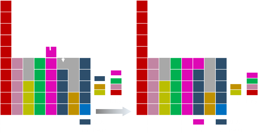
On the first pass we pull off the top items from each list. Here they are the dark and light blue elements. We move sufficient of the dark over to the light. After the move, the dark blue elements remaining are less then 1.0 so this is added to the small list. We've now completed one column. We know the alias for this column and the probability.
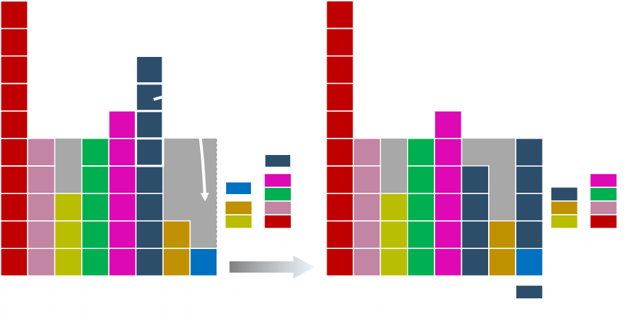
On this pass, the dark blue is the top item on the small list, and the magenta the top item on the large list. The magenta stays on the large list after the donation.
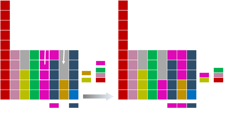
The magenta is still on the top of the large list and is paired with the orange. After the shift, the magenta moves to the small list.
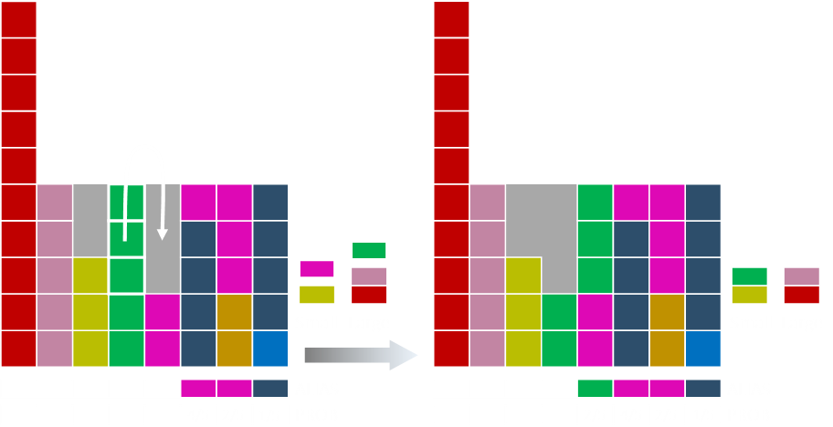
Some of the green moves over to fill the magenta. Green is then added to the short list.
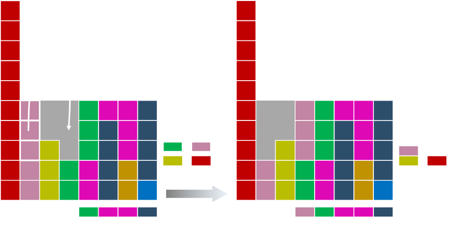
Some of the salmon coloured bar moves over.
Some of the red moves over.
And the last of the red bar
Finally we run the clean up loop setting anything left in the large list to one.
Result
Once the two arrays (PROB, ALIAS) have been generated, selecting the random element is easy (and quick). First a fair n-sided die is rolled to determine the proposed value (selecting the column). Either this value is kept (with the probability in the PROB array for that column), or it's switched to the value in the ALIAS array.
I hope you agree that this is pretty neat algorithm!